Playground · research instrument
DSP · AudioAcoustics Calculators
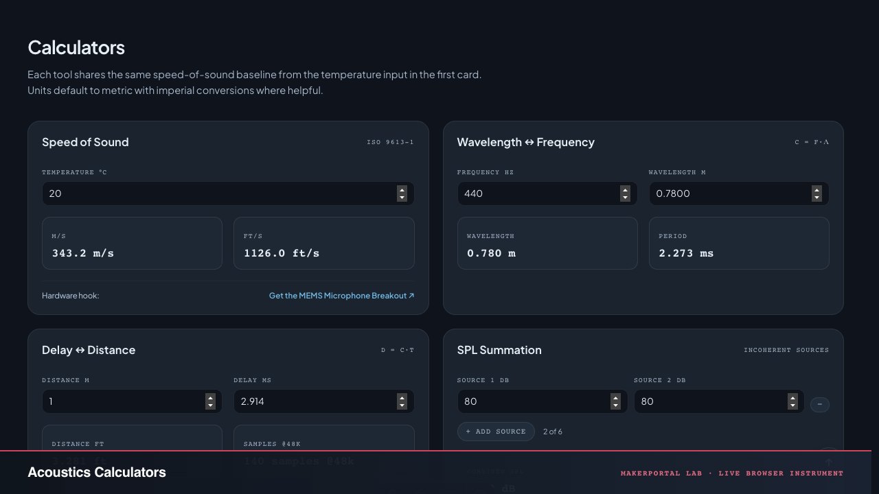
Speed of sound, wavelength, delay, SPL summation, dB/ratio conversion, RT60, Helmholtz resonance, Doppler shift, Mass Law (TL), and NR Curves — essential acoustic tools in one place.
Independent research instrument — not claimed as MakerPortal shipped product code. Methods, equations, assumptions, and limitations are disclosed so you can inspect what the page does and does not establish.
Calculators
Each tool shares the same speed-of-sound baseline from the temperature input in the first card. Units default to metric with imperial conversions where helpful.
Wavelength ↔ Frequency
c = f·λ0.780 m
2.273 ms
Delay ↔ Distance
d = c·t3.281 ft
140 samples
SPL Summation
incoherent sources83.0 dB
dB ↔ Ratio Converter
voltage / pressure & power1.995
6.00 dB
RT60 — Sabine & Eyring
room acoustics60.0
0.69 s
0.63 s
214 Hz
0.57 m
Helmholtz Resonance
bass-reflex port + cavity37.8 Hz
Port Length Calculator
speaker box tuning8.5 cm
Doppler Shift
moving source & observerPositive velocity means moving towards each other.
1030.0 Hz
Mass Law (STC est.)
transmission loss32.8 dB
NR Curve Limits
iso 1996 limits79 dB
63 dB
52 dB
45 dB
39 dB
35 dB
32 dB
30 dB
28 dB
Essence
Every knob here is physics you can point at. Temperature sets how fast molecules shove each other, that sets wavelength, that sets whether your room is a closet or a cave at 40 Hz.
Sound isn't mysterious. It's air acting like a spring. Cold air is sluggish, hot air is snappy, a speaker cone moves and the shove travels at . If you know , you know the size of a wave, how long it takes to cross a stage, whether two speakers add or fight, and how long a room holds onto a clap. These calculators share one baseline because in real life they do — same air, same day.
Method & limitations
Speed of sound — why hot rooms are faster
From kinetic theory: where , is gas constant, molar mass, K. For dry air at 1 atm this collapses to ISO 9613-1:
At 20 C that's 343.2 m/s. Picture O2 and N2 darting faster when warm — a pressure pulse gets handed off quicker. Humidity makes lighter so rises less than 0.5% even at 100% RH / 40 C, negligible for audio alignment. Pressure itself cancels: denser but also stiffer. This feeds wavelength, delay, and Helmholtz cards. If you leave temperature at 20 C while your venue is 30 C, your delay is about 1.7% short — 17 mm per metre of path, audible as comb in line-array rigs.
Wavelength ↔ Frequency ↔ Period
The wave repeats every , so it must satisfy
That's it. No hidden constant. A 440 Hz A is about 0.78 m — about a guitar body. 20 Hz is 17 m, bigger than most rooms, which is why bass pressurizes instead of propagates. 20 kHz is 17 mm, smaller than a tweeter dome, which is why it beams. If speaker spacing is greater than , you get spatial aliasing; if a port is less than , lumped models still work. Keep that mental ruler handy.
Delay ↔ Distance
Time of flight is trivial but central:
1 ms is 34.3 cm at 20 C. Haas says less than 30 ms arrivals fuse; greater than 50 ms they echo. For alignment, match subs and mains within 0.5 ms at crossover — about 17 cm. The calculator also gives samples at 48 kHz because your DSP delay line lives in samples, not meters. Temperature matters again: a summer outdoor stage needs 2% less electrical delay than winter.
SPL Summation — incoherent power, not pressure
Sound level meters read pressure squared averaged over time. Intensities add for uncorrelated sources (two drummers, two HVAC units). So convert each dB back to power, sum, convert back:
Equal sources: . Two 80 dB incoherent = 83.0 dB. Ten = 90 dB. If perfectly coherent and in-phase (same signal, same wire), pressures add linearly:
That gives +6 dB per doubling. Reality lives between — correlated low-frequency room modes give almost +6, diffuse mid frequencies +3. Don't blindly add decibels.
dB ↔ Ratio — why 20 vs 10
Decibel is always 10 log of a power ratio. Power scales as amplitude squared. So for field quantities (pressure , voltage , velocity):
Inversions: Doubling power = 10 log10 2 = +3.01 dB. Doubling pressure = 20 log10 2 = +6.02 dB. Same physical change, different bookkeeping because power goes as . Voltage gain in audio follows 20 log; amplifier power follows 10 log. Toggle matters — 6 dB vs 3 dB mistakes blow drivers.
RT60 — Sabine vs Eyring, the honest story
Sabine (1898) imagined energy sloshing uniformly, losing a tiny fraction A/S per bounce. Mean free path 4V/S, reflections per second cS/4V, exponential decay . Set dB:
0.161 = 55.26/c ~ — it's just unit conversion for 60 dB and . Works for live rooms.
Eyring (1930) fixes high absorption by not approximating . Treat energy as geometric series: after reflections . Solve for 60 dB drop:
When , and Eyring tends to Sabine. When , Eyring can be 2x shorter — and more realistic. Both ignore air absorption (about 0.01 dB/m at 2 kHz, grows as ), frequency-dependent , and non-diffuse geometry. That's why real rooms measured with swept sine differ by plus or minus 20%.
Two derived tools: room constant and critical distance. is where direct equals reverberant field — beyond it you hear room, not speaker. is source directivity. Schroeder's crossover:
Below you hear individual eigenmodes as booms; above, a smooth decay. Constant 2000 assumes about 10 modes overlap within a half-power bandwidth — rules of thumb vary 1500 to 4000, we pick 2000. Use it to know when to fix geometry vs add absorption.
Helmholtz & Port Length — the bottle as spring-mass
Blow across a bottle: air plug in neck is mass , cavity volume is spring with compliance . Resonance of that mass-spring:
End correction because moving air extends past physical ends, and each end adds its own: 0.85r for an end flush with a wall (flanged; Rayleigh's radiation reactance, 8/3π rounded) and 0.6133r for a bare tube end (free; Levine and Schwinger). A port has one of each, the outer end flush with the baffle and the inner end free in the box: with , the 0.732·D of most port formulas. Both ends flanged gives L+1.7r; both free gives L+1.23r. Both cards here use 1.4633r.
Inversion for box tuning: That's the port length card. Assumptions: , (lumped), circular unflared port, rigid lossless walls, no fill. Real ports with flare act longer at high SPL (end correction changes with velocity), fibrous damping material raises the box's apparent volume (it makes the air compress more nearly isothermally, so a stuffed box acts larger and tunes slightly lower), and driver Vas adds compliance. Start here, then measure and trim by 15%.
Doppler Shift — wavefronts chasing their source
If source moves toward observer, each crest is emitted from a closer point — wavelengths compress. Observer moving toward meets crests faster. For source toward observer, observer toward source (positive toward each other):
If , denominator goes to 0 and — boom, shock forms. Negative means receding, drops pitch. At audio speeds (10 m/s car is 3% of ) shift is about 0.3 semitones per 10 m/s — subtle but Doppler for rotating Leslie horn at 5 m/s rim speed is why it choruses. Keep from temperature to avoid phantom cents.
Mass Law & NR Curves — transmission and comfort
A limp wall's inertia resists being driven by sound. Random-incidence transmission loss for single leaf:
dB
surface mass kg/m2, Hz. 6 dB per octave, 6 dB per doubling mass — mass times frequency law. Real panels dip at coincidence where bending wave matches trace wavelength; above that stiffness helps again. Double-leaf adds mass-spring-mass resonance. Use Mass Law as upper bound for limp, heavy, damped walls.
NR (Noise Rating) ISO 1996: linear curves where indexes octave band 31.5 Hz to 8 kHz, tabulated constants. Your measured octave SPL must sit below the curve to claim that NR. NR 25 is concert hall, 35 bedroom, 45 open office. It's a single-number mask for annoyance and speech interference, not a physical law.
Playbook — how to actually use this
Speaker alignment in 60 s
Measure air temp, set top card. Enter physical distance between subs and tops in delay card — read ms and 48k samples. Flip: enter your DSP's ms to see distance. Keep within 0.5 ms at crossover.
Room quick-check
Put your room L,W,H and average 0.15 furnished. Note Schroeder . Below , use mode analyzer; above, use absorption. If critical distance is less than listening distance, you hear more room than direct — move closer or add absorption.
Box tuning without guessing
Want 38 Hz from 30 L with 5 cm dia port: enter in Helmholtz or port-length card. Get cm effective, so cut cm. Cut 5% long, measure the impedance minimum between the two peaks, trim. If chuffing, increase area and recalc — scales as for same .
Noise target
Pick NR 35 for a studio aircon limit, read grid for allowed SPL per octave. If 500 Hz band breaks the curve, that's HVAC midband whine — treat it first. If low bands break, it's rumble — mass law tells you how much wall mass you need.
What this is not
No air absorption in RT60, no frequency-dependent , no non-rectangular rooms, no modal coupling, no port nonlinearity or driver compliance shift, no coincidence or double-leaf TL, no humidity correction for unless you want it. These are design-estimate instruments — verified against Sabine, Eyring, and lumped Helmholtz, but validated against measurement in your air, your box, your walls.
Anatomy of the instrument
Eleven calculators, one shared physics engine. Here is what each card does, how the script ties them together, and why the temperature input sits at the top of the page.
The shared engine
- 01
Temperature as the root node. The top card computes via ISO 9613-1. Every other calculator reads this single
currentCvariable — wavelength, delay, Helmholtz, port length, and Doppler all depend on it. Change temperature and every card recalculates in one pass, because in the real world you don't get different speeds of sound in different formulas. - 02
Event-driven recalculation. There is no polling loop. Each input's
inputevent fires a targeted update function. The temperature handler fans out to six dependent calculators; the others trigger just their own readouts. ThewlUpdatinganddelayUpdatingflags prevent infinite circular updates when wavelength↔frequency or distance↔delay inputs drive each other bidirectionally. - 03
SPL dynamic rows. The summation card starts with two sources and lets you add up to six via a DOM factory. Each new row gets an input listener and a remove button wired at creation time. Renumbering keeps labels consistent when you delete from the middle. The
splSumArrayfunction converts each dB to linear power, sums, then converts back — the same math a sound level meter does internally. - 04
dB mode toggle. The dB↔ratio converter switches between 20·log (voltage/pressure) and 10·log (power). Changing the radio fires
updateFromDb()which recomputes both fields from the current dB input value. The visual density card gives you both sides at once so you can spot-check which convention applies.
Central equation — c(T)
Every result on this page — wavelength, delay, Helmholtz resonance, Doppler shift — traces back to this one line. At 20 °C it's 343.2 m/s; at 30 °C it's 349.0 m/s. That is 1.7%, and 1.7% of a metre is 17 mm of path — audible as comb filtering in multi-speaker arrays. Set temperature first.
RT60, Helmholtz, and the bigger cards
- 05
RT60 dual-output. Both Sabine and Eyring compute in parallel from the same dimensions and α. The Sabine formula uses directly; Eyring uses instead. They diverge at high absorption because Sabine's small-α approximation breaks. Critical distance and Schroeder frequency derive from whichever RT60 is finite — the dashboard uses Sabine preferentially for the Schroeder constant.
- 06
Helmholtz ↔ Port Length duality. These two cards are inverses of each other. Helmholtz takes port diameter, port length, and cavity volume → gives resonance frequency. Port length takes box volume, port diameter, and target tuning → gives required length. Both use the same end correction, (one end flush with the baffle, one free inside the box). If you enter the output of one as the input of the other, the numbers should agree — a built-in sanity check.
- 07
Doppler shift sign convention. Positive velocity means moving toward each other — source velocity is + when source approaches observer, observer velocity is + when observer approaches source. This matches the standard physics convention . If you set source velocity to negative (receding), frequency drops instead of rises.
- 08
NR curve grid. The nine octave bands (31.5 Hz to 8 kHz) are hard-coded ISO 1996 constants. Each band's allowed SPL = . The grid updates all nine cells when you change the target NR level. If you're measuring a room, compare each octave band against the grid — any band exceeding the limit means the room fails that NR rating, even if other bands are quiet.
- 09
Mass Law baseline. The transmission loss calculator uses the limp-wall formula . It's accurate to about ±3 dB for single-leaf homogeneous panels above the critical frequency. Below coincidence, stiffness resonance dominates instead of mass — this tool assumes you're above that region.
- 10
No idle compute. The page initializes once via
initAcousticCalculators(), guarded by adata-initflag to prevent re-init on Astro page transitions. No setInterval, no requestAnimationFrame. The only computation happens on user input events. Zero CPU while you read the method section.
Gear behind this build
DSP audio · 23 picks
Audio measurement & monitoring23
 $159.00Headphones
Audio-Technica ATH-M50X Professional Studio Monitor Headphones, Black, Professional Grade, Critically Acclaimed, with Detachable Cable
Reference monitoring headphones used for akous's binaural audio testing.
 Microphone
BEHRINGER ECM8000
Reference omni for acoustic measurement — captures the same pressure field these fast calculators approximate with ray-tracing and modal sums.
 $229.00Audio interface
Behringer UMC1820 Audiophile 18x20 USB Audio/MIDI Interface with Midas Mic Preamplifiers and ADAT I/O | For Recording Microphones and Instruments
Audio interface used building Biquadia — 8-preamp USB I/O for real-time DSP testing.
 $180.00Microphone
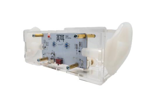
Bit Trade One BIMIMI - Binaural Stereo Microphone Easy BINAURAL Recording/ASMR/Podcast/Recording/Streaming / W7.2×H1.9×D2.6 inches/ADBMM
Binaural stereo mic capturing HRTF — the spatial cues this head-tracked panner approximates via ITD/ILD and quaternion yaw driving StereoPannerNode.
 $54.99Microphone
Blue Yeti Nano Premium USB Microphone - Shadow Grey (Renewed)
Compact USB condenser mic used for nymic testing.
 $9.99Audio
Comimark 1Pcs ADMP401 MEMS Microphone Breakout Module Board for Arduino Universal 1.3cm*1cm
MEMS mic breakout used for real-time DSP experiments feeding into Biquadia.
 $59.98Microphone
Dayton Audio EMM-6 Precision Omnidirectional Electret Condenser Microphone for Room Acoustic Analyzers and Audio Measurement Systems, Calibration Data File with Response Graph Included
Omni condenser with cal file — pair with REW to measure SPL, RT60, and comb filtering the acoustic calculator suite computes via image-source method.
 $49.99Microphone
Dayton Audio iMM-6C Calibrated Measurement USB-C Microphone for iPhone, iPad Tablet and Android,Black
USB-C calibrated mic for iPhone/iPad — take to listening room and verify room-mode eigenfrequencies against calculator's mode list up to 300Hz.
 $124.97Microphone
Dayton Audio UMM-6 USB Measurement Microphone
Legacy USB measurement mic for REW — capture on-axis SPL and compare to enclosure designer frequency response with baffle diffraction.
 Microphone
Dayton Audio UMM-6 USB Measurement Microphone
USB cal mic for nearfield SPL and cone-breakup waterfall — capture the CSD breakup modes this simulator predicts via modal superposition.
 $39.98Tool
Focusound 24 Packs Acoustic Foam Panels Pyramid 2" X 12" X 12", Soundproofing Foam Noise Cancelling Foam with 120 PCS Double-Side adhesive
Pyramid foam taming room modes at f = n c / 2L — measure RT60 drop and compare to acoustic-calculator predictions for absorption coefficient vs frequency.
 $39.99Tool
Focusound 50 Pack Acoustic Foam Panels 1" x 12" x 12" Sound Proof Foam Panles Soundproofing Noise Cancelling Wedge Panels for Home Office Recoding Studio with 300PCS Double-Side Adhesive
1-inch wedge for mid-high absorption — use with room-mode calculator's Sabine RT60 equation to predict reverberation time reduction.
 Audio interface
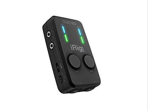
IK Multimedia iRig Pro Duo I/O USB audio interface, TRS balanced & headphones outputs, audio mixer to 24-bit, midi interface for music studio, recording, podcasting, streaming & social apps
Portable 2-channel USB-C audio interface used for mobile Biquadia field recording.
 $135.00Book
Immersive Sound: The Art and Science of Binaural and Multi-Channel Audio (Audio Engineering Society Presents)
Derives HRTF, ITD = d/c sinθ, and head-tracking compensation — the exact panning law this playground interpolates as you drag yaw.
 $38.38Book
Master Handbook of Acoustics, Seventh Edition
Bible of RT60, Sabine, and absorption coefficients — the exact formulas these acoustic calculators implement for reverb, room modes, and critical distance.
 $149.95Microphone
miniDSP UMIK-1 Calibrated Measurement Microphone
Calibrated USB mic with individual cal file — measure your room's RT60 and modal peaks to validate the room-mode eigenfrequencies this calculator predicts.
 $135.99Apparatus
MJDHS Professional Ernst Chladni Vibration Generator, Chladni Pattern, and Visual Sound Wave are Classic Experimental Tools in The Field of Acoustics and Vibration(30hz-20khz, 30w)(Size:6.5in/6.5in)
30W driver sweeping through plate resonances — matches the eigenvalue sweep in this Chladni lab where sand flees antinodes to settle on nodal lines.
 $168.00Microphone
RØDE NT-USB+ Professional-Grade USB Condenser Microphone for Recording
USB condenser mic used for nymic testing.
 $8.99Audio
SABRENT USB External Stereo Sound Card Adapter, Plug & Play (AU-MMSA)
USB audio interface used in early Biquadia MEMS-mic prototyping.
 Microphone
Sennheiser Pro Audio Sennheiser Pro Audio Wireless Microphone System, Black (MKE600)
Wireless mic system used for akous's ambient/binaural field recording.
 $319.00Microphone
Shure MV7+ USB-C & XLR Podcast Dynamic Mic with Stand - Black
USB/XLR hybrid mic used building and testing nymic.
 $237.00Microphone
Shure MV88+ USB-C Video Kit Stereo Condenser Microphone
Portable stereo condenser mic kit used for Biquadia field/video capture.
 $98.00Headphones
Sony MDR7506 Professional Large Diaphragm Headphone
Reference studio headphones used for akous's binaural audio testing.
Prices shown were retrieved from the Amazon Product Advertising API on 8 October 2026 and are indicative only — the price and availability on Amazon at the time of purchase apply.
More gear across every app: the full Gear list →
Two gotchas worth knowing
Decibel addition without coherence check
This page adds dB sources incoherently — 10·log sum of powers. That's right for independent noise sources, separate HVAC vents, or uncorrelated drivers. But if you're summing two outputs of the same DSP carrying the same signal, and they're wired in phase, pressure adds linearly — the result is up to 6 dB higher per doubling, not 3 dB. The calculator has no way to know your coherence scenario. Always ask: are these independent sources or two copies of the same signal?
Temperature drift across cards
The temperature input sits in the first card and every other calculator reads currentC reactively. If you change temperature, all dependent cards recompute. But if you enter dimensions first and then change temperature before noting the earlier results, you may not realize the wavelength and delay numbers you just read have shifted underneath you. Always confirm temperature before taking critical measurements — a 10 °C error is a 1.7% error in c, which propagates to every derived quantity on the page.
Hardware Rigs & Field Notes
Hardware build / Mic arrays
Real-Time Acoustic Beamforming on an iPhone with miniDSP UMA-8
Live SRP-PHAT direction finding, superdirective MVDR beamforming on a 44 mm ring, and physical directivity limits.
Hardware build / Measurement
Headphone Measurement with a Binaural Head: HD 650 + UMC1820
HATS measurement rig, true-RMS multimeter calibration under load, and per-ear swept-sine transfer functions.
JavaScript — the core solver
The acoustics library underpinning all calculators on this page. Copy-paste speedOfSound and splSumArray into any audio tool — they have zero dependencies and the same math as a $UMC1820-equipped measurement rig uses internally.
Core acoustics — JavaScript
const speedOfSound = (tC) => 331.3 * Math.sqrt(1 + tC / 273.15);

const splSumArray = (levels) => {
  let sum = 0;
  for (const L of levels) sum += Math.pow(10, L / 10);
  return 10 * Math.log10(sum);
};

const wavelength = (f, c) => c / f;

const frequencyFromWavelength = (wl, c) => c / wl;

const delayFromDistance = (d, c) => (d / c) * 1000;

const distanceFromDelay = (ms, c) => (ms / 1000) * c;

const rt60Sabine = (V, A) => {
  if (A <= 0) return Infinity;
  return 0.161 * V / A;
};

const rt60Eyring = (V, S, alpha) => {
  if (alpha <= 0 || alpha >= 1) return Infinity;
  return 0.161 * V / (-S * Math.log(1 - alpha));
};

const schroederFrequency = (V, T60) => {
  if (T60 <= 0) return Infinity;
  return 2000 * Math.sqrt(T60 / V);
};

const criticalDistance = (Q, R) => {
  if (R <= 0) return Infinity;
  return Math.sqrt(Q * R / (16 * Math.PI));
};

// End corrections per open end, in neck radii: flush with a wall (flanged)
// and free (a bare tube end). A port has one of each: 1.4633 r = 0.732 D.
const END_CORRECTION_FLANGED = 0.85;
const END_CORRECTION_FREE = 0.6133;
const PORT_END_CORRECTION = END_CORRECTION_FLANGED + END_CORRECTION_FREE;

const helmholtzFrequency = (S, L, V, c = 343, endCorrection = PORT_END_CORRECTION) => {
  const Leff = L + endCorrection * Math.sqrt(S / Math.PI);
  if (Leff <= 0 || V <= 0) return 0;
  return (c / (2 * Math.PI)) * Math.sqrt(S / (V * Leff));
};

const portLength = (Sp, fb, Vb, c = 343, endCorrection = PORT_END_CORRECTION) => {
  if (fb <= 0 || Vb <= 0) return 0;
  const k = (2 * Math.PI * fb) / c;
  return Sp / (k * k * Vb) - endCorrection * Math.sqrt(Sp / Math.PI);
};

const dopplerShift = (f, vs, vo, c) => vs >= c ? Infinity : f * (c + vo) / (c - vs);

const massLawTransmissionLoss = (mass, f) => mass > 0 && f > 0 ? Math.max(0, 20 * Math.log10(mass * f) - 47.2) : 0;Lead magnet · Privacy-first
Export current calculator state as a reference card
One click generates a timestamped report of all eleven calculator values above as a clean text reference — useful for studio notes, client deliverables, or sharing your tuning state with a colleague. Enter your email to unlock the clean export (no watermark). Free watermarked version always available. Privacy-first: email stays in your browser localStorage, optional newsletter via Buttondown (no tracking pixels, D-014 compliant).
Email stored in localStorage · RSS at /rss.xml
Frequently asked questions
Which RT60 formula should I trust — Sabine or Eyring?
For average absorption below 0.2 (most furnished rooms) they nearly agree, so either is fine. Once ᾱ exceeds 0.3, Eyring is more physically correct because Sabine overestimates the number of reflections per second. Real measured RT60 typically falls between the two — use Sabine as a conservative upper bound and Eyring as the physics-consistent lower bound.
Why do two 80 dB sources sum to 83 dB, not 86 dB?
Two independent noise sources are incoherent — their instantaneous pressures aren't correlated. You add intensities (power), not pressures. 10·log₁₀(10⁸ + 10⁸) = 10·log₁₀(2×10⁸) ≈ 83.0 dB. If they were perfectly in phase and coherent (same signal on two identical speakers wired together), you'd get +6 dB instead — but that only happens in controlled setups, not with independent sources.
What is Schroeder frequency and why does it matter?
It divides your room into two acoustic regimes. Below fs, room eigenmodes are sparse and audible as discrete booms — that's where you need modal treatment. Above fs, modes overlap so densely they blend into a smooth decay — that's where broadband absorption works. The tool computes it from volume and RT60 using fs = 2000·√(T₆₀/V).
Does humidity affect my delay calculations?
Negligibly for timing. At 40 °C and 100% RH, speed of sound rises only about 0.5%. Your 1 ms delay would be off by 0.005 ms — far below what a DSP delay line can resolve. Temperature matters far more: from 20 °C to 30 °C, c rises from 343.2 to 349.0 m/s — 1.7%, so a wavefront covers 1.7% more ground in the same time. Over one metre of path that is 17 mm, which is audible as comb filtering in multi-speaker arrays.
How do I use the port length calculator and actually build from it?
Enter box volume, desired tuning frequency, and port diameter. The calculator gives you the physical length with both end corrections taken out: the outer end flush with the baffle and the inner end free inside the box. Build the port 10% longer than the computed value, install it, measure the impedance curve with your audio interface (the box tuning is the minimum between its two peaks), then trim to exact length. A port that's too long tunes lower than predicted; too short tunes higher. PVC pipe with a hose clamp is forgiving for prototyping.
Shareable still
The instrument, captured—not illustrated.
This 16:9 frame is rendered from the real browser instrument above. It is the page's canonical preview for image search, link unfurls, and posts that need to show what the tool actually does.
Download 1280 × 720 JPEG