Playground · research instrument

Live Earth

A rotating globe with real data underneath it — actual coastlines, an astronomically accurate day/night line, real current weather, and the ISS tracked from its real orbital elements. Drag to spin.

Independent research instrument — not claimed as MakerPortal shipped product code. Methods, equations, assumptions, and limitations are disclosed so you can inspect what the page does and does not establish.

Day / Night

The terminator and lighting are updated continuously from your clock using the Sun’s apparent position and Greenwich sidereal time.

Live UTC: —
Subsolar point: —

Hardware hook:Get the MOVA Globe Satellite View with Cloud Cover (4.5 inch) ↗

What's real here, and what isn't

A globe looks simple until you ask where each pixel comes from. This one has four independent data pipelines — only one runs purely in your browser. Here is what is real, what is simplified, and where the math lives.

Coastlines

Real geometry, self-hosted

Natural Earth 110m public-domain polygons, converted to GeoJSON and served from /data/world-land-110m.json. No live fetch to a map tile server. Projection is d3.geoOrthographic with clipAngle $90^\circ$ , scale tied to canvas radius, updated on drag. We intentionally draw at low precision $0.1^\circ$ to keep frame rate while staying recognizable. Toggle wireframe vs filled — same geometry, two strokes.

Day / Night

Real astronomy from your clock

No API. We compute subsolar latitude $\delta$ and longitude $\lambda_s$ from Julian Date $JD$ . Steps: $T = (JD - 2451545)/36525$ , mean longitude $L$ , mean anomaly $M$ , equation of center $C(M)$ , apparent longitude, obliquity $\epsilon$ , right ascension $\alpha = \text{atan2}(\cos\epsilon \sin\lambda, \cos\lambda)$ , declination $\delta = \arcsin(\sin\epsilon \sin\lambda)$ . Greenwich sidereal time from same $JD$ gives subsolar longitude.

Terminator is the great circle $s \cdot p = 0$ where $s$ is sun vector, $p$ is surface point. We build orthonormal basis $u, v \perp s$ and sweep $p(t)=\cos t \, u + \sin t \, v$ , $t \in [0,2\pi)$ . Night shading is per-pixel $s \cdot n < 0$ where $n$ is surface normal reconstructed from canvas $x,y$ plus viewer depth $\sqrt{1 - x^2 - y^2}$ . Dot product sign decides day vs night, alpha ramps with $-|s\cdot n|$ . That is why terminator is not a hard line but soft with grazing illumination.

This is exact to $\sim0.01^\circ$ for modern dates — more than enough to watch sunset sweep across continents as you drag.

Weather

Real observations, static snapshot

Sixteen cities, real current conditions from Open-Meteo at build time, committed as src/data/weather.json with generatedAt. Refresh script hits weather API every 4 hours via GitHub Action, writes static JSON, no runtime fetch from browser. That avoids API keys in client and makes demo deterministic.

Temperature to color is piecewise linear interpolation through stops $-15^\circ$ to $40^\circ$ C: deep blue $\to$ cyan $\to$ green $\to$ amber $\to$ red. Dot placed by projecting $(\phi,\lambda)$ through same orthographic projection. Hidden behind globe if $p_z < 0$ after rotation — d3-geo path returns null for backside, so cities disappear naturally as Earth spins, same as satellites.

Limitation: snapshot in time, not forecast. If you open at night and see $32^\circ$ C in Mumbai, that was current at last refresh, not predicted.

ISS Tracker

Real TLE, simplified propagator

TLE from CelesTrak, also scraped every 4 hours to src/data/satellite.json. Line 1 contains epoch yyddd.ddd, line 2 contains $i, \Omega, e, \omega, M_0, n$ in deg, deg, dimensionless, deg, deg, rev/day.

We parse $n$ rad/s, get semi-major axis $a = (GM / n^2)^{1/3}$ from Kepler third law, $GM=398600.4418$ km $^3$ /s $^2$ . Mean anomaly at now $M = M_0 + n \Delta t$ , solve Kepler $M = E - e \sin E$ by Newton iteration (15 iters), true anomaly $\nu = 2 \text{atan2}(\sqrt{1+e}\sin(E/2), \sqrt{1-e}\cos(E/2))$ , radius $r = a(1-e\cos E)$ . Perifocal to inertial via $R(\Omega)R(i)R(\omega)$ , then ECEF via GMST rotation $\theta$ .

That is two-body Keplerian. Full SGP4 adds $J_2$ oblateness, drag term $B^*$ , lunar-solar perturbations, resonance. We omit those for footprint and clarity — no 1000-line SGP4 port. Result drifts $\sim$ few km vs truth within hours of epoch, fine for "watch it move" but not for pass prediction or docking. For precision, use satellite.js SGP4. Trail is recomputed -25 min to now every second, projected as LineString so it clips at horizon like coastlines.

Honesty ledger

Coastlines — real shapes, fake shading. Orthographic is geometric idealization; no terrain, no atmosphere scattering.
Day/night — real sun position, simplified scattering. Night texture is a procedurally tinted alpha mask, not city lights database.
Weather — real temps at snapshot, not live, not forecast, 16 points only — spatial interpolation would be misleading so we show dots only.
ISS — real TLE epoch, simplified physics. Accuracy badge: illustrative <10 km near epoch, degrades as $\Delta t$ grows, no maneuver modeling.

Anatomy of the globe

Three independent data pipelines drive one canvas. Here is what each pixel is actually doing.

The render pipeline

01
d3.geoOrthographic projection. The globe uses d3-geo's orthographic projection with clipAngle 90°, centered at (φ₀ = 18° tilt, λ₀ = variable spin). scale is tied to canvas radius. No WebGL — every line is drawn with Canvas 2D via d3.geoPath. Precision is 0.1° per d3 projection property, keeping tessellation light for smooth drag at 60 fps.
02
Coastlines from Natural Earth. 110m-resolution public-domain polygons served from /data/world-land-110m.json, fetched once at init with an AbortController for cleanup. Drawn as geopaths — wireframe mode strokes them, filled mode fills them. Day/night mode uses 0.72 opacity; weather/ISS modes dim to 0.4 to keep data layers legible.
03
Day/night painting. Every half-second, subsolar declination δ and longitude λ_s are computed from the Julian Date using the Astronomical Almanac formula. A 256×256 off-screen canvas pre-computes per-pixel sun-dot-product: for each visible disk pixel, the surface normal is reconstructed from screen (x,y) plus viewer depth, dotted with the sun vector. Negative dot = night, positive = day, with an alpha ramp for grazing illumination at the terminator edge. This is redrawn only when the solar minute changes or lambda0 shifts ≥ 0.2°.

Terminator great circle construction

\text{Terminator} = \{ \mathbf{p} \mid \mathbf{s} \cdot \mathbf{p} = 0 \}, \quad \mathbf{p}(t) = \cos t \, \mathbf{u} + \sin t \, \mathbf{v}

Basis vectors u, v are orthonormal and perpendicular to sun direction s. The 180-point sweep traces the sunrise/sunset line across the globe. This line is what you see as the red curve — the exact boundary between illuminated and dark hemispheres.

Data overlays and interaction

01
Weather mode. 16 cities with real current conditions from Open-Meteo, baked at build time into weather.json. Temperature maps to color via piecewise linear interpolation through 5 stops (−15°C deep blue → 40°C red). Cities are drawn as filled circles with white stroke through d3.geoPath.pointRadius(5). Backside cities are automatically hidden by d3-geo returning null for dots behind the globe.
04
ISS tracker. Real TLE from CelesTrak, refreshed every 4 hours via GitHub Action. Two-body Keplerian propagation: mean anomaly M = M₀ + nΔt, solve M = E − e sin E via 15 Newton iterations, compute true anomaly ν and radius r, rotate from perifocal to ECEF via R(Ω)R(i)R(ω) and GMST. Trail is a −25-minute-to-now LineString recomputed once per second.
05
Auto-rotation and drag. The globe spins at 2.4°/s by default. Dragging pauses auto-rotation (lambda0 updates from pointer delta). An IntersectionObserver pauses the rAF loop when the canvas is off-screen to save CPU. ThemeObserver on data-theme triggers redraw for dark/light mode.

Gear behind this build

Earth & orbital mechanics stack · 8 picks

Orbital hardware8

$399.98Model

LEGO 92176 Ideas NASA Apollo Saturn V Space Rocket and Vehicles, Spaceship Collectors Building Set with Display Stand [Amazon Exclusive], 14+ years

1:110 Saturn V with 1969 Apollo stages — build it while your virtual ship undergoes Lorentz contraction and relativistic Doppler shift of CMB to visible blue.

$399.98 USDView ↗

$28.95Model

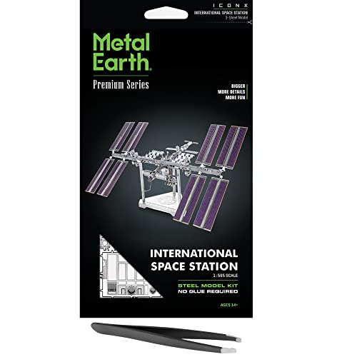
Metal Earth Fascinations Premium Series International Space Station 3D Metal Model Kit Bundle with Tweezers

Steel ISS model — track the real ISS live on this globe's TLE orbit, then hold the model while it passes over your city at 7.66 km/s orbital velocity.

$28.95 USDView ↗

$399.00Model

Motorized Metal Solar System Model Kit, 600+ Precision Parts Mechanical Orrery with LED Sun, STEM Astronomy Engineering Building Kit for Adults, Planetary Gear Planetarium Desk Display

600+ precision metal parts, motor-driven planets on brass gear trains — a buildable mechanical computer tracing the same Newtonian choreography this page integrates with symplectic Yoshida 4th order.

$399.00 USDView ↗

$249.00Apparatus

MOVA Self Rotating Globe, Earth with Clouds Classic (4.5")

Solar-powered, self-rotating satellite globe that spins continuously using ambient light and Earth's magnetic field — demonstrating Coriolis torque and gyroscopic rotation live.

$249.00 USDView ↗

$74.01Book

Orbital Mechanics for Engineering Students: Revised Reprint (Aerospace Engineering)

Derives n-body equations, figure-eight choreography existence proof, and symplectic energy conservation — exactly the trajectory this page verifies stays bounded for 500 periods.

$74.01 USDView ↗

$39.99Model

Replogle Ready to Assemble Illuminated World 12" Diameter Globe, USA Cartography, Modern Acrylic Stand and Blue Ocean Globe Ball. Easy to assemble globe that shows both Political and Vegetative information including political borders and provincial borders, major ocean currents, detailed lakes, rivers, tributaries and canals. (Illuminated)

Backlit globe with constellation overlay — compare its static terminator to this page's dynamically computed solar declination and real-time weather overlay across 16 cities.

$39.99 USDView ↗

$57.75Book

Satellite Orbits: Models, Methods and Applications

SGP4 and TLE propagation — this globe computes ISS position client-side from real TLE elements using the same Kepler + J2 math Montenbruck derives.

$57.75 USDView ↗

$31.63Book

Visual Differential Geometry and Forms: A Mathematical Drama in Five Acts

Sequel to Visual Complex Analysis — explains how conformal warp preserves infinitesimal circles, which you see as grid squares stay square under holomorphic f(z).

$31.63 USDView ↗

Prices shown were retrieved from the Amazon Product Advertising API on 19 July 2026 and are indicative only — the price and availability on Amazon at the time of purchase apply.

More gear across every app: the full Gear list →

Two gotchas worth knowing

Orthographic depth clipping

d3.geoOrthographic with clipAngle 90° correctly omits geometry on the back half of the globe, but it does this per path segment — not per point. A long LineString that wraps around the back will be clipped into multiple visible arcs on the front. This is mathematically correct but can look like the ISS trail "jumps" when a portion of it moves behind the globe. The trail is re-sampled every second, so the jump smooths out.

Two-body drift vs SGP4

The ISS propagator is two-body Keplerian — it ignores J₂ oblateness (which rotates the orbital plane ~5°/day), atmospheric drag (which lowers altitude ~2 km/month during solar max), and third-body perturbations. Within 1-2 hours of the TLE epoch, the position is within a few kilometers. Past 12 hours, the error grows to tens of kilometers. The readout says "illustrative, not precision tracking" for this reason.

Copyable: subsolar point & ISS propagation

The two real physics cores powering the globe — drop directly into any JS visualization.

JavaScript — subsolar point (declination, longitude)

function subsolarPoint(date) {
  const jd = date.getTime() / 86400000 + 2440587.5;
  const T = (jd - 2451545.0) / 36525;
  const meanLon = ((280.46646 + T * (36000.76983 + 0.0003032 * T)) % 360 + 360) % 360;
  const M = ((357.52911 + T * (35999.05029 - 0.0001537 * T)) % 360 + 360) % 360;
  const eqCtr = Math.sin(M) * (1.914602 - T * (0.004817 + 0.000014 * T));
  const appLon = meanLon + eqCtr - 0.00569;
  const obliquity = 23.439291 - 0.0130041667 * T;
  const ra = Math.atan2(Math.cos(obliquity) * Math.sin(appLon), Math.cos(appLon));
  const decl = Math.asin(Math.sin(obliquity) * Math.sin(appLon));
  const gmst = 280.46061837 + 360.98564736629 * (jd - 2451545.0);
  return { decl, lon: ra - gmst };
}

JavaScript — ISS two-body Keplerian propagation

const GM = 398600.4418; // km^3/s^2

function propagate(elems, dateMs) {
  const dtSec = (dateMs - elems.epochMs) / 1000;
  let M = elems.meanAnom0 + elems.nRadS * dtSec;
  M = ((M % (2 * Math.PI)) + 2 * Math.PI) % (2 * Math.PI);
  let E = M;
  for (let i = 0; i < 15; i++)
    E -= (E - elems.ecc * Math.sin(E) - M) / (1 - elems.ecc * Math.cos(E));
  const nu = 2 * Math.atan2(Math.sqrt(1 + elems.ecc) * Math.sin(E / 2),
                           Math.sqrt(1 - elems.ecc) * Math.cos(E / 2));
  const r = elems.a * (1 - elems.ecc * Math.cos(E));
  const xOrb = r * Math.cos(nu), yOrb = r * Math.sin(nu);
  // Rotate perifocal → inertial → ECEF
  const theta = gmstRad(dateMs);
  const xEcef = xOrb * cos(theta) + yOrb * sin(theta);
  const yEcef = -xOrb * sin(theta) + yOrb * cos(theta);
  const zEcef = zOrb; // … full rotation matrix in page script
  const rMag = Math.hypot(xEcef, yEcef, zEcef);
  return {
    lat: Math.asin(zEcef / rMag) * 180 / Math.PI,
    lon: Math.atan2(yEcef, xEcef) * 180 / Math.PI,
    alt: rMag - 6378.137,
  };
}

Frequently asked questions

How accurate is the day/night terminator?

The terminator is computed from the Sun's apparent position using Julian Date, solar declination, and Greenwich sidereal time — the same astronomical formulas used in planetarium software. It is accurate to ~0.01° for modern dates, more than enough to watch sunset sweep across continents. The night shade is a per-pixel dot-product between the surface normal and sun vector, producing a soft transition rather than a hard line.

Why does the ISS trail sometimes clip at the horizon?

The ISS trail is a LineString projected through d3.geoOrthographic with clipAngle 90°. Points behind the globe (p_z < 0) are automatically omitted by d3-geo, so the trail appears to wrap around the visible hemisphere. This is the same mechanism that hides cities and coastlines on the back side of the Earth.

Is the ISS position accurate enough for pass prediction?

No. This simulation uses simplified two-body Keplerian propagation from real TLE elements — it omits J₂ oblateness, atmospheric drag (B* term), and lunar-solar perturbations that full SGP4 includes. Within a few hours of the TLE epoch, the error is a few kilometers. For precision tracking, use satellite.js SGP4. This demo is for watching it move, not for scheduling telescope passes.

How is weather data updated?

Weather data is fetched from the Open-Meteo API at build time via a GitHub Action that runs every 4 hours, commits the result to src/data/weather.json, and triggers a redeploy. No API keys in the client, no live fetch from the browser. The temperature-to-color mapping is a piecewise linear interpolation through five color stops from −15°C (deep blue) to 40°C (red).

Why does the globe spin and can I control it?

The globe auto-rotates at 2.4°/second by default, giving a continuous view of all longitudes. You can pause rotation with the "Pause rotation" button, drag left/right to spin manually (horizontal drag maps to longitude delta × 0.3), and toggle between wireframe and filled rendering. The IntersectionObserver pauses the animation loop when the canvas is off-screen to save battery.

Shareable still

The instrument, captured—not illustrated.

This 16:9 frame is rendered from the real browser instrument above. It is the page's canonical preview for image search, link unfurls, and posts that need to show what the tool actually does.

Download 1280 × 720 JPEG

Live Earth — live MakerPortal instrument screenshot — Canonical capture · real UI · no generated scientific artwork

Continue the experiment

All lab instruments →

Research

Live Earth

What's real here, and what isn't