Playground · research instrument

Lattice Boltzmann Wind Tunnel

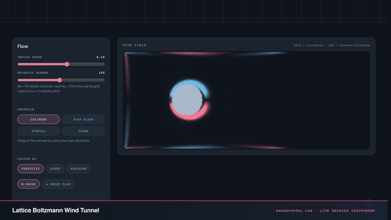
A real-time 2D wind tunnel running a D2Q9 lattice Boltzmann solver. Place a cylinder, plate, or airfoil in the stream and turn up the Reynolds number until the steady wake destabilizes into a shedding Von Kármán vortex street. Colour the flow by vorticity, speed, or pressure — and paint your own obstacles right on the canvas.

Independent research instrument — not claimed as MakerPortal shipped product code. Methods, equations, assumptions, and limitations are disclosed so you can inspect what the page does and does not establish.

Flow

Inflow speed0.10Reynolds number150

Re ≳ 90 sheds vortices; near Re = 300 the coarse grid nears its ω → 2 stability limit.

Obstacle

Drag on the canvas to paint your own obstacle.

Colour by

viscosity ν
—

relaxation ω
—

effective Re
150

steps
0

status
running

Hardware hook:Get the Windsible Desktop Wind Tunnel ↗

Flow field

blue = clockwise · red = counter-clockwise

Method & limitations

Each node carries nine populations on the D2Q9 stencil. Every step they collide — relaxing toward the equilibrium at rate ω — then stream to neighbours. Solid cells reflect populations by full-way bounce-back. The inflow is a fixed-velocity boundary, the outflow is zero-gradient, and vorticity is the discrete curl of the recovered velocity field. In the low-Mach limit this recovers incompressible Navier–Stokes with ν = cₛ²(τ − ½).

D2Q9 velocity set

e_i \in \{(0,0),\ (\pm1,0),\ (0,\pm1),\ (\pm1,\pm1)\}

Lattice Boltzmann equation (collide + stream)

f_i(\mathbf{x} + \mathbf{c}_i\Delta t,\ t + \Delta t) = f_i(\mathbf{x}, t) - \frac{1}{\tau}\bigl[f_i(\mathbf{x}, t) - f_i^{eq}(\mathbf{x}, t)\bigr]

BGK equilibrium (second-order Hermite expansion)

f_i^{eq} = w_i\,\rho\left[1 + 3(\mathbf{c}_i\!\cdot\!\mathbf{u}) + \frac{9}{2}(\mathbf{c}_i\!\cdot\!\mathbf{u})^2 - \frac{3}{2}|\mathbf{u}|^2\right]

D2Q9 weights

w_0 = \frac{4}{9},\quad w_{1-4} = \frac{1}{9},\quad w_{5-8} = \frac{1}{36}

Kinematic viscosity

\nu = c_s^2(\tau - \tfrac{1}{2})\Delta t,\qquad c_s = \frac{1}{\sqrt{3}}

Reynolds to relaxation

Re = \frac{U\cdot D}{\nu}\quad\Longrightarrow\quad \tau = 3\nu + \tfrac{1}{2} = \frac{3UD}{Re} + \tfrac{1}{2}

CFL-like stability constraint

\tau > 0.5,\qquad \omega = \frac{1}{\tau} \in (0.5,\ 2.0)

Macroscopic (conserved moments)

\rho = \sum_{i=0}^{8} f_i,\qquad \mathbf{u} = \frac{1}{\rho}\sum_{i=0}^{8} f_i\,\mathbf{c}_i

What is real physics

Mass and momentum are conserved by the collision (unit-tested), the wake instability and shedding frequency emerge on their own, and the Reynolds-number dependence is genuine — not a scripted animation.

What it simplifies

A coarse grid, single-relaxation-time BGK, weak compressibility, and staircased bounce-back walls. It is quantitatively rough at high Re and near ω = 2, and is not a validated finite-volume/finite-element CFD code.

The solver lives in src/lib/fluid-lbm.ts (D2Q9 equilibrium, BGK collision, bounce-back, streaming), unit-tested for the velocity-set moments, equilibrium moment recovery, and mass/momentum conservation.

Anatomy of the instrument

Every pixel above answers to the math below. Here is what each piece of the visualization and control panel is actually doing, and why it is built that way.

The flow canvas

01
Grid geometry. $240 \times 96$ lattice nodes with $x$ horizontal and $y$ vertical. The y-axis is flipped for rendering so positive-y points up (physics convention), while canvas row zero sits at the visual top.
02
Colour modes. Vorticity maps clockwise rotation to blue and counter-clockwise to red. Speed ramps black → blue → red with the inflow speed as scale. Pressure draws low-pressure regions in blue and high-pressure in red, computed from the density field via $\Delta p \propto (\rho - 1)$ .
03
Obstacle rendering. Solid cells are filled with a muted neutral tone distinct from the flow palette. Drag-to-paint uses a brush radius of 3 lattice units with a circular mask, and obstacles are communicated to the solver as a single $Uint8Array$ mask that triggers bounce-back and skips collision.
04
Pixel-perfect ImageData rendering. The colour map writes directly into a Uint8ClampedArray backed by the canvas ImageData, then blits in one putImageData call per frame. No texture uploads, no WebGL — just a raw pixel buffer, perfectly matching the lattice resolution.
05
Inflow and outflow boundaries. The left column and top/bottom rows are forced to the uniform inflow equilibrium (Dirichlet). The right column copies the second-to-last column (zero-gradient Neumann outflow). The long sides wrap periodically via the stream step's modulo indexing.

Collision and stream — one full step

f_i(\mathbf{x}+\mathbf{c}_i\Delta t,\ t+\Delta t) = f_i(\mathbf{x},t) + \Omega_i,\qquad \Omega_i = -\frac{1}{\tau}\bigl[f_i(\mathbf{x},t) - f_i^{eq}(\mathbf{x},t)\bigr]

Collide → bounce-back → stream → re-impose boundaries. That four-step sequence runs six times per animation frame, giving approximately 360 lattice steps per second at 60 fps.

Controls, readouts, and LBM machinery

01
Inflow speed slider. Sets the x-velocity $u_0$ at the left boundary in lattice units. When Reynolds is fixed, changing the speed updates $\omega$ implicitly because $\nu = UD/Re$ . When you then move the Re slider, it recomputes $\omega$ from that expression.
02
Reynolds number slider. Computes kinematic viscosity from $\nu = (u_0 \cdot D) / Re$ using the cylinder diameter $D$ , then derives $\omega = 1/(3\nu + 0.5)$ and clamps it to $[0.5, 1.96]$ . You are sliding the physics parameter directly — not a visual effect multiplier.
03
Obstacle presets. Cylinder is a filled circle (radius ≈ 16% of channel height). Flat plate is a vertical line segment. Airfoil is a tilted teardrop with angle of attack −0.28 rad, tapered toward the trailing edge. Clear zeroes the mask and resets the flow.
04
Play, pause, reset. Pause freezes the solver loop — the canvas holds the last rendered frame. Reset re-initialises every node to the uniform inflow equilibrium and clears the step counter. State persists across mode changes.
05
Readouts and render loop. The live panel shows $\nu$ (viscosity), $\omega$ (relaxation rate), step count, and status. Six LBM steps run per rAF frame. A stability guard checks the midpoint cell after each batch: if $\rho$ is NaN, $>5$ , or $<0.1$ , the flow auto-resets and the status line reports the reason.

Gear behind this build

CFD & LBM stack · 5 picks

Fluid dynamics5

$78.83Book

An Introduction to Fluid Dynamics (Cambridge Mathematical Library)

Derives Navier-Stokes and Reynolds number Re = UL/ν — crank Re past ~50 in this LBM tunnel and watch the von Kármán vortex street Batchelor describes appear.

$78.83 USDView ↗

$85.23Book

Fluid Mechanics

Boundary layer separation and drag coefficient Cd vs Re — place cylinder in LBM tunnel and validate wake Strouhal against White's drag crisis curve.

$85.23 USDView ↗

$299.00Kit

FUN-TECH-LAB Windsible, Desktop Wind Tunnel, for 1:64 Diecast Car Models, Miniature Wind Simulation, Display Stand, for Collectors and Hobbyists

Tabletop wind tunnel with flow-visualization streamlines — park a 1:64 model in the test section and compare the real wake against this page’s D2Q9 vorticity field and Strouhal estimate.

$299.00 USDView ↗

$57.87Book

The Lattice Boltzmann Method: Principles and Practice (Graduate Texts in Physics)

Defines the D2Q9 equilibrium distribution f_i^eq = w_i ρ [1 + c_i·u/cs² ...] and BGK collision operator this tunnel implements live for Von Kármán shedding.

$57.87 USDView ↗

$73.94Book

Turbulent Flows

Kolmogorov energy cascade and vortex stretching — crank Reynolds number in LBM tunnel past transition and see Pope's -5/3 law emerge in vorticity power spectrum.

$73.94 USDView ↗

Prices shown were retrieved from the Amazon Product Advertising API on 19 July 2026 and are indicative only — the price and availability on Amazon at the time of purchase apply.

More gear across every app: the full Gear list →

Two gotchas worth knowing

τ > 0.5 or crash

The relaxation time $\tau$ must exceed 0.5 — otherwise the effective viscosity $\nu = c_s^2(\tau - 0.5)$ becomes zero or negative and the scheme is unconditionally unstable. At $\tau = 0.5$ ( $\omega = 2.0$ ) the collision just overwrites populations with equilibrium every step; numerical round-off cannot dissipate, and high-frequency modes grow without bound. The practical ceiling is around $\omega \approx 1.96$ ( $\tau \approx 0.51$ ) — beyond that, lattice-scale oscillations (chequerboard modes) contaminate the solution. Raise the Reynolds slider until the flow resets and you have hit the limit.

Compressibility artifacts

LBM is weakly compressible by construction — pressure fluctuations propagate as acoustic waves at speed $c_s = 1/\sqrt{3}$ , giving an effective Mach number of $Ma \approx 0.1-0.2$ in this setup. It is not a true incompressible Navier–Stokes solver. At higher Reynolds numbers the density variations become visible in the pressure colour mode, and at the stability limit they can trigger the auto-reset guard. This is a deliberate trade-off: true incompressibility would require a pressure-Poisson solve at each step, which would consume far more CPU than the lightweight collisional scheme running here.

TypeScript, the collision-stream core

The full solver is in src/lib/fluid-lbm.ts. Below is the essential collision-stream loop — the equilibrium function, BGK relaxation, and the macroscopic moment recovery. Drop it into any TypeScript codebase alongside the D2Q9 constants and it runs.

D2Q9 equilibrium + BGK collision

export const CX = [0, 1, 0, -1, 0, 1, -1, -1, 1];
export const CY = [0, 0, 1, 0, -1, 1, 1, -1, -1];
export const W = [4/9, 1/9, 1/9, 1/9, 1/9, 1/36, 1/36, 1/36, 1/36];
export const CS2 = 1 / 3;

export function equilibrium(rho: number, ux: number, uy: number,
  out: Float64Array | number[]): void {
  const usq = 1.5 * (ux * ux + uy * uy);
  for (let i = 0; i < 9; i++) {
    const cu = 3 * (CX[i] * ux + CY[i] * uy);
    out[i] = W[i] * rho * (1 + cu + 0.5 * cu * cu - usq);
  }
}

// Inside collide(): for each lattice cell c
//   rho = sum_i f[i][c]
//   ux  = (1/rho) * sum_i CX[i] * f[i][c]
//   uy  = (1/rho) * sum_i CY[i] * f[i][c]
//   for i in 0..8: f[i][c] += omega * (eq[i] - f[i][c])

// stream(): periodic wrap in a temp buffer, then swap
// bounceBack(): swap opposite pairs inside solid cells (1↔3, 2↔4, 5↔7, 6↔8)

Frequently asked questions

What is the Lattice Boltzmann Method?

Instead of solving the Navier–Stokes equations directly, LBM tracks nine discrete populations of fictitious particles on each lattice node (the D2Q9 stencil). Every step the populations relax toward a local equilibrium (BGK collision) and then hop to neighbouring nodes (streaming). In the low-speed limit this mesoscopic bookkeeping provably reproduces incompressible Navier–Stokes flow, and it is beautifully parallel and simple to code.

What is the D2Q9 velocity set?

D2Q9 means two spatial dimensions and nine discrete velocities per node: a rest particle (0,0), four cardinal links at (±1,0) and (0,±1), and four diagonal links at (±1,±1). Together they guarantee fourth-order isotropy of the lattice tensors — necessary and sufficient to recover the Navier–Stokes stress tensor in the continuum limit. The nine weights are 4/9 for rest, 1/9 for cardinals, and 1/36 for diagonals.

What does BGK single-relaxation-time collision mean?

BGK (Bhatnagar-Gross-Krook) collision approximates the full Boltzmann collision integral by a linear relaxation toward local equilibrium: fᵢ ← fᵢ + ω(fᵢᵉq − fᵢ). All nine populations relax at the same rate ω = 1/τ. It is the simplest collision operator that still conserves mass and momentum. More advanced operators (multi-relaxation-time, entropic) improve stability at high Reynolds numbers but add significant computational cost.

How are Reynolds number and viscosity linked in this simulation?

Reynolds number Re = U·D/ν, where U is the inflow speed, D the obstacle diameter, and ν the kinematic viscosity. In LBM, ν = c_s²(τ − 0.5)Δt with c_s² = 1/3 in lattice units. The slider computes τ from your chosen Re via ω = 1/(3ν + 0.5). Raise Re → lower ν → ω moves toward 2.0 (the stability ceiling). At Re ≳ 300 on this 240×96 grid, ω ≈ 1.96 and lattice artefacts emerge.

What are the practical limits of this simulation?

It is a genuine mesoscopic solver — not a decorative animation — but it is deliberately lightweight. It runs single-precision on a coarse 240×96 grid with simple bounce-back (staircased) obstacle boundaries, single-relaxation-time BGK, and weak compressibility (Ma ~ 0.1). Quantitatively it is rough at high Re and near ω = 2, and it is not a substitute for a validated finite-volume CFD code. A stability guard monitors the midpoint cell density and auto-resets the flow if it diverges.

Shareable still

The instrument, captured—not illustrated.

This 16:9 frame is rendered from the real browser instrument above. It is the page's canonical preview for image search, link unfurls, and posts that need to show what the tool actually does.

Download 1280 × 720 JPEG

Lattice Boltzmann Wind Tunnel — live MakerPortal instrument screenshot — Canonical capture · real UI · no generated scientific artwork

Continue the experiment

All lab instruments →

Research

Lattice Boltzmann Wind Tunnel

Flow

Method & limitations