Playground · research instrument

Chladni Plate Simulator

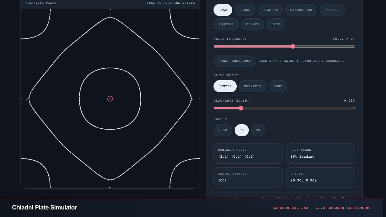
Bow a metal plate covered in sand and the grains flee the vibrating regions, collecting along the silent nodal lines. This is the same experiment as a driven modal superposition: sweep the frequency, move the driver, and watch thousands of grains assemble the resonant geometry.

Independent research instrument — not claimed as MakerPortal shipped product code. Methods, equations, assumptions, and limitations are disclosed so you can inspect what the page does and does not establish.

Sound made visible

Running. Drag anywhere on the plate to move the driver; grains re-settle onto the new nodal lines.

Vibrating plateDrag to move the driver

Drive frequency10.00 × f₁

slow upward glide through every resonance

Drive point

Resonance width γ0.030

Grains

Dominant modes: —
Mode share: —
Grains settled: —
Driver: —

Hardware hook:Get the 3B Scientific Metal Square Chladni Plate 7 inch ↗

The math under the sand

Cosines, resonance denominators, and gradient drift — every grain of sand follows the same three equations. Here they are in full, the same expressions the solver evaluates every 1/120th of a second.

The driven modal superposition

A plate driven at a point $(x_0,y_0)$ responds as a weighted sum of its standing-wave modes. The weight is the product of the mode shape at the drive point and a resonance curve — enormous when the drive frequency sits on that mode's eigenfrequency, tiny elsewhere:

Driven response at every grid cell

u(x,y) = \sum_{m,n} \frac{\phi_{mn}(x_0,y_0)\,\phi_{mn}(x,y)}{\sqrt{(f_{mn}^2 - f^2)^2 + (\gamma f f_{mn})^2}}

Where $\phi_{mn}(x,y) = \cos(m\pi x)\cos(n\pi y)$ with free-edge (Neumann) boundary conditions. The drive point $(x_0,y_0)$ sets each mode's coupling: placing the driver on a mode's nodal line zeroes that mode entirely. Moving the driver genuinely re-weights the sum.

Plate dispersion — why the slider is logarithmic

\frac{f_{mn}}{f_1} = \frac{m^2 + n^2}{2}

Bending waves in a stiff plate obey $\omega \propto k^2$ , unlike a membrane's $\omega \propto k$ . Resonances spread quadratically: the gap from mode $(1,0)$ to $(2,0)$ is smaller than from $(7,0)$ to $(8,0)$ . The frequency slider is a $\log_2$ scale for this reason — it compresses the octaves so you can sweep the whole audible range linearly by hand.

Two modes like $(4,2)$ and $(2,4)$ share an eigenfrequency on a square plate because $m^2+n^2$ is symmetric. At resonance they respond together, and their superposition creates the diagonal symmetry of the classic star pattern. This degeneracy is not a coding shortcut — it is the physics of symmetry, the same reason a circular plate has richer patterns than a square one.

How the sand actually moves

The grains are not decoration; they are the measurement. Vibrating regions kick grains into a random walk whose step size grows with local amplitude, while the time-averaged bounce drifts them down the amplitude gradient:

Stochastic grain transport (Grabec-style)

d\mathbf{x} = -\mu\,\nabla(u^2)\,dt + \sigma|u|\,d\mathbf{W}

Deterministic drift down the squared-amplitude gradient ( $\mu = 0.12$ ) plus amplitude-scaled jitter ( $\sigma = 0.006$ ), capped at $0.004$ per step in plate-normalized units. Integrated at a fixed $\frac{1}{120}$ s timestep independent of display frame rate — the same timestep the grid solver uses.

Why it works everywhere at once

Both effects — jitter and gradient drift — vanish exactly where $u=0$ (the nodal lines) and scale with $|u|$ . That is why the silent curves are the only places grains can come to rest: any grain that lands on a node experiences zero kick and zero drift, so it stays. Any grain off a node gets pushed. After a few seconds thousands of grains self-organize into the eigenfunction geometry — no pattern database, no lookup table.

Separable evaluation

Because $\phi_{mn}(x,y)=\cos(m\pi x)\cos(n\pi y)$ is separable, the $144\times144$ grid is rebuilt from pre-computed cosine tables — each cell is a pure multiply-add with no trig calls. The $16$ strongest modes per frequency are kept, and a smoothstep blend fades discrete jumps over $0.7$ s so the grains never teleport.

The response amplitude is auto-normalized so patterns stay visible between resonances. Grain–grain collisions are ignored (the real physics involves avalanche-like piling at nodes, which is visually interesting but computationally separate). Cosine modes are exact for a free membrane and a standard approximation for a free plate — a real plate's biharmonic eigenfunctions bend the lines near edges. Patterns are qualitatively faithful; eigenfrequencies of any physical plate will differ.

Anatomy of the simulator

Every grain, every grid cell, and every readout traces back to the modal superposition and the stochastic transport model. Here is what each piece is doing and why it is built that way.

The canvas and its grains

01
The plate. A $640\times640$ HiDPI canvas with up to $2\times$ device-pixel scaling. Each grain is a $2\times2$ px filled rectangle — deliberately not a particle system with sprites. At 5,000 grains the browser draws 10,000 rects per frame, which is trivial for the Canvas API and leaves the CPU for the physics step.
02
The driver marker. A ring-and-crosshair drawn at $(x_0, y_0)$ in the theme's CTA color. Dragging anywhere on the plate moves it; the pointToPlate() function normalizes pointer coordinates to $[0,1]$ plate units. Keyboard arrows nudge it at $0.02$ or $0.05$ (shift) per press — the same precision a finger gives.
03
The field overlay. Toggled via "Show field", it is a $145\times145$ imageData rendered on an offscreen canvas — one texel per grid cell, CTA-colored, alpha proportional to $|u|$ . It rebuilds only when the grid changes (not per frame) and shares the same fade-blend as the physics field, so it never disagrees with what the grains feel.
04
The render loop. Fixed $\frac{1}{120}$ s physics step via an accumulator pattern decoupled from frame rate (capped at 8 steps per frame). An IntersectionObserver pauses the sim when the canvas leaves the viewport. The loop never spins idle — it only ticks when visible and unpaused.

Controls and readouts

01
Frequency slider. Logarithmic $\log_2(f)$ scale from $2^{-0.32}\approx 0.8\times f_1$ to $2^{6.15}\approx 71\times f_1$ , spanning the first $8\times8$ mode pairs. Presets snap to named resonances like star $(4,2)/(2,4)$ and rosette $(6,2)/(2,6)$ . The slider is continuous — any fractional $\log_2$ value produces a valid superposition.
02
Resonance width $\gamma$ . Controls the denominator in the resonance curve: small $\gamma$ gives sharp, isolated modes; large $\gamma$ blends neighbors. At the default $0.03$ , the star preset shows clean degenerate mixing; at $0.12$ the same frequency produces a mushy blend with adjacent modes leaking in.
03
Drive point buttons. Center $(0.5,0.5)$ excites only symmetric modes; off-axis $(0.353,0.278)$ breaks symmetry and reveals asymmetric patterns; edge $(0.5,0.02)$ simulates bowing the plate rim. The cross preset uses edge drive specifically to flip the sign of $(2,0)$ coupling relative to $(0,2)$ — the same physics, mathematically different superposition.
04
Grain count. 2.5k, 5k, or 9k particles. The transport model is $O(N)$ — each grain independently samples the field and steps. At 9k on mobile the physics loop stays under budget because the grid evaluation is cheap (bilinear lookup into pre-computed arrays). Changing grain count re-initializes all positions randomly.
05
Readouts. Dominant modes lists the top 3 mode pairs by coefficient magnitude (degenerate partners folded together). Mode share shows the leading mode's percentage of total coefficient weight. Grains settled samples every $N$ -th grain and counts those with $|u| < 0.1u_{max}$ — effectively, grains on or near a node. Driver shows the current $(x_0, y_0)$ coordinates.

Gear behind this build

Cymatics stack · 5 picks

Cymatics hardware5

$31.75Apparatus

3B Scientific U56006 Metal Square Chladni Plate, 7" Length x 7" Width

Precision steel plate for cymatics — dust with fine sand and drive at computed eigenfrequency to realize the Bessel-function nodal patterns this simulator solves.

$31.75 USDView ↗

$279.56Kit

GSC International WVGENKIT Standing Wave Demonstration Kit for Physical Science

Driver + square plate kit — sweep frequency and see nodal lines accumulate sand along Chladni figures exactly as this modal eigensolver's Laplacian eigenmodes predict.

$279.56 USDView ↗

$136.62Apparatus

MJDHS Professional Ernst Chladni Vibration Generator, Chladni Pattern, and Visual Sound Wave are Classic Experimental Tools in The Field of Acoustics and Vibration(30hz-20khz, 30w)(Size:6.5in/6.5in)

30W driver sweeping through plate resonances — matches the eigenvalue sweep in this Chladni lab where sand flees antinodes to settle on nodal lines.

$136.62 USDView ↗

$100.39Book

The Physics of Musical Instruments

Modal analysis of plates and strings with Bessel functions — root of Chladni plate eigenmodes and waveguide modal cutoff fc = c/2a this toolbox computes.

$100.39 USDView ↗

$Toysmith Euler’s Disk Desk Toys Office Adults - Create Hypnotic Light Refraction Sound Display - Science Decor Home And Workspace - Kinetic Motion Physics Models Kids 8+$ $44.99Apparatus

Toysmith Euler’s Disk Desk Toys Office Adults - Create Hypnotic Light Refraction Sound Display - Science Decor Home And Workspace - Kinetic Motion Physics Models Kids 8+

Spinning disk's decreasing contact and rising audible frequency demonstrate modal energy concentration — same standing-wave energy argument explaining why Chladni sand avoids vibrating regions.

$44.99 USDView ↗

Prices shown were retrieved from the Amazon Product Advertising API on 19 July 2026 and are indicative only — the price and availability on Amazon at the time of purchase apply.

More gear across every app: the full Gear list →

Two gotchas worth knowing

Cosine modes approximate, not exact

A free plate obeys the biharmonic equation, not the Helmholtz equation. Its eigenfunctions are not pure $\cos(m\pi x)\cos(n\pi y)$ — they bend near the edges in ways cosine modes cannot capture. This sim produces qualitatively faithful Chladni patterns, but the exact curvature of nodal lines near boundaries and the eigenfrequencies themselves differ from any physical plate. If you build a real Chladni rig, expect the frequencies to be shifted and some patterns to look slightly warped.

Degenerate modes share the work

On a square plate, $(m,n)$ and $(n,m)$ are always at the same eigenfrequency. Both respond together and the resulting pattern is their superposition — not "one of them won." The metrics readout folds degenerate partners into one entry so you see the combined effect. If you see diagonal symmetry in a pattern, it is almost always coming from a degenerate pair, not from a single mode with unusual shape.

The solver, copyable

The two functions behind every grain on this page. The first computes the mode coefficients from a drive frequency and point — the heart of the modal superposition. The second advances the sand grains along the amplitude gradient with stochastic jitter.

computeCoefficients + stepPhysics

const modeFreq = (m, n) => (m * m + n * n) / 2;

function computeCoefficients(f) {
  const all = [];
  for (let m = 0; m <= MAX_MODE; m++) {
    for (let n = 0; n <= MAX_MODE; n++) {
      if (m === 0 && n === 0) continue;
      const fmn = modeFreq(m, n);
      const coupling = Math.cos(m * Math.PI * driveX)
                     * Math.cos(n * Math.PI * driveY);
      const denom = Math.hypot(fmn * fmn - f * f, gamma * f * fmn);
      const c = coupling / denom;
      if (Math.abs(c) > 1e-9) all.push({ m, n, c });
    }
  }
  all.sort((a, b) => Math.abs(b.c) - Math.abs(a.c));
  const kept = all.slice(0, COEFF_KEEP);
  const floor = kept.length ? Math.abs(kept[0].c) * 1e-3 : 0;
  return kept.filter(k => Math.abs(k.c) >= floor);
}

function stepPhysics() {
  const umax = blendedUMax(), inv = 1 / umax;
  for (let p = 0; p < grainCount; p++) {
    const s = sampleField(px[p], py[p]);
    const un = s[0] * inv;
    const drift = -MU * 2 * un * inv * PHYSICS_DT;
    let dx = drift * s[1]
           + JITTER * Math.abs(un) * (Math.random() - 0.5);
    let dy = drift * s[2]
           + JITTER * Math.abs(un) * (Math.random() - 0.5);
    dx = Math.min(STEP_CAP, Math.max(-STEP_CAP, dx));
    dy = Math.min(STEP_CAP, Math.max(-STEP_CAP, dy));
    let nx = px[p] + dx, ny = py[p] + dy;
    if (nx < 0) nx = -nx; else if (nx > 1) nx = 2 - nx;
    if (ny < 0) ny = -ny; else if (ny > 1) ny = 2 - ny;
    px[p] = nx; py[p] = ny;
  }
}

Frequently asked questions

What are Chladni patterns?

Chladni patterns are the visible geometry of standing waves. When you vibrate a plate at a resonant frequency, regions of high vibration amplitude eject sand, while the nodal lines — the curves where amplitude is zero — collect it. The sand traces out the eigenfunctions of the plate. Different frequencies excite different mode shapes, each with a distinct pattern of intersecting nodal lines.

Why do some modal patterns look the same or share symmetry?

On a square plate, the modes (m,n) and (n,m) share the same eigenfrequency because f ∝ m² + n². When the drive excites a degenerate frequency, both modes respond simultaneously and their superposition creates a new pattern — often with diagonal symmetry. The (4,2) and (2,4) pair produces the classic star-shaped pattern, not either mode alone. This degeneracy is not a bug: it is why a square plate has richer patterns than a rectangular one.

What does the resonance width γ control?

γ sets how sharply the plate responds to being slightly off resonance. A small γ (0.01) isolates a single mode: you must hit its exact eigenfrequency or the plate stays nearly silent. A large γ (0.12) blends neighboring modes together, creating broader, less distinct patterns. Think of it as the Q-factor of the plate — high Q means narrow, sharp resonance peaks.

Why does moving the drive point change the pattern?

Each mode's amplitude depends on the product φₘₙ(x₀,y₀) × φₘₙ(x,y). The first factor is the mode shape evaluated at the drive point. If you place the driver on a nodal line of a particular mode — a line where that mode's amplitude is zero — that mode cannot be excited at all. Move the driver away and the mode comes back. This is why off-axis drive creates asymmetric patterns: it selectively suppresses modes symmetric about the new position.

What is the difference between a Chladni plate and a drum membrane?

Chladni plates are driven by a vibrating point source and the plate itself supports bending waves where ω ∝ k². A drum membrane stretches under tension and obeys a different wave equation where ω ∝ k. The pattern families differ: plate modes spread out quadratically (f ∝ m² + n²), membrane modes linearly (f ∝ √(m² + n²)). The plate has richer, denser patterns, and the eigenfrequencies are not integer multiples of the fundamental — which is why the slider uses a log scale.

Shareable still

The instrument, captured—not illustrated.

This 16:9 frame is rendered from the real browser instrument above. It is the page's canonical preview for image search, link unfurls, and posts that need to show what the tool actually does.

Download 1280 × 720 JPEG

Chladni Cymatics — live MakerPortal instrument screenshot — Canonical capture · real UI · no generated scientific artwork

Continue the experiment

All lab instruments →

Research

Chladni Plate Simulator

Sound made visible