Playground · research instrument

N-Body Orbital Choreography

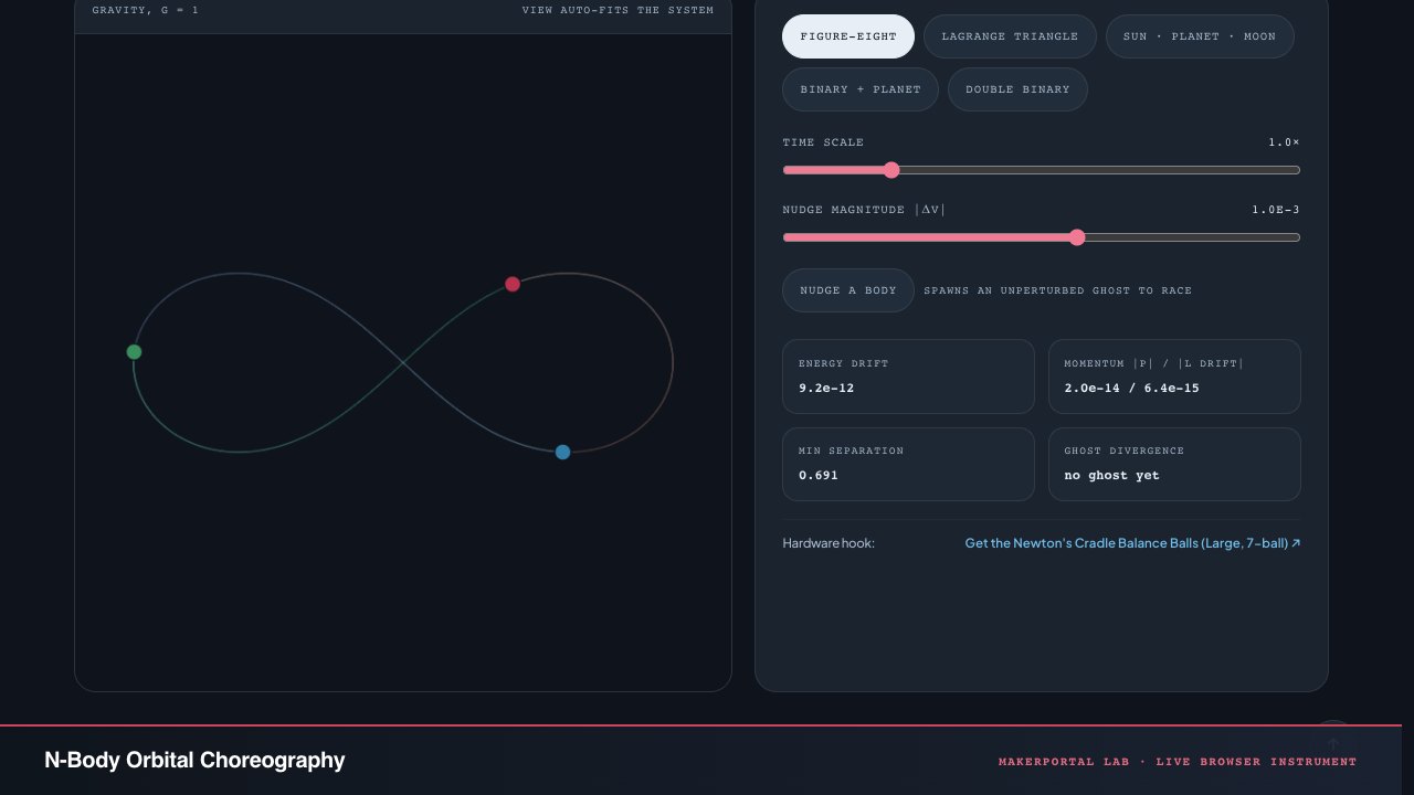
In 2000, Chenciner and Montgomery proved three equal masses can chase each other forever around a figure-eight. It exists in real gravity — this page integrates it live with a symplectic scheme accurate enough to hold the dance for hundreds of orbits, then lets you nudge it and watch how long the choreography survives.

Independent research instrument — not claimed as MakerPortal shipped product code. Methods, equations, assumptions, and limitations are disclosed so you can inspect what the page does and does not establish.

A stable dance, until you touch it

Running. Nudge a body and a faint ghost keeps dancing the unperturbed choreography for comparison.

Gravity, G = 1View auto-fits the system
spawns an unperturbed ghost to race
Energy drift
Momentum |P| / |L drift|
Min separation
Ghost divergence

Why the integrator matters more than the forces

Newtonian gravity between three bodies has no general closed-form solution — this is the original chaos problem. Ordinary integrators (like RK4) leak energy steadily, so an orbit that should repeat forever spirals in or escapes as pure numerical artifact. A symplectic integrator instead conserves a slightly-perturbed energy exactly, so the error stays bounded for hundreds of periods instead of accumulating.

The figure-eight is special: it is a proven periodic solution, and mildly stable — tiny perturbations wobble around it rather than destroying it instantly. The Lagrange triangle is its opposite: an exact solution that is linearly unstable for equal masses. The integration here is clean enough that the triangle holds until you seed the instability yourself — nudge it, then watch the same |δv| that barely dents the figure-eight tear the triangle apart. That asymmetry is real physics, not integration error.

Integration scheme

Yoshida 4th-order composition of velocity Verlet, dt = 2·10⁻³

Three Verlet sub-steps with weights (w₁, w₀, w₁), w₀ = −∛2·w₁. Validated: figure-eight returns to its start after one period (T ≈ 6.3259) to within 10⁻⁴, energy drift ~10⁻¹¹ over 50 periods.

Collision safety

r² → r² + ε², ε² = 10⁻⁶

Plummer softening caps the force during close encounters so the integration never blows up. At choreography distances (~1) it shifts positions by less than 10⁻⁴; the min-separation readout tells you when it is actually active.

Conserved quantities

E = Σ ½mv² − Σ mᵢmⱼ/rᵢⱼ, P = Σ mv, L = Σ m(r × v)

All three are monitored live and shown without smoothing. Initial conditions are shifted to the center-of-momentum frame, so |P| should sit at machine precision.

Honest limitations

Fixed-step integration loses accuracy during very close encounters (the softening is what keeps it finite); a production ephemeris would switch to adaptive or regularized steps. Everything is planar (2D), and the ghost comparison shares the same integrator — it measures sensitivity to the nudge, not absolute truth.

Anatomy of the simulation

Five preset systems, one symplectic integrator, and a ghost twin that never gets nudged. Here is what each piece of the simulation actually does under the hood.

The integrator and physics core

  1. 01

    Yoshida 4th-order symplectic composition. Three Verlet sub-steps per full step with weights [w₁, w₀, w₁] where w₀ = −∛2 · w₁, w₁ = 1/(2 − ∛2). Each sub-step is a standard velocity Verlet: half-kick, drift, half-kick. The composition cancels error terms up to O(dt⁴) while preserving the symplectic structure. dt = 2 × 10⁻³ in dimensionless time units.

  2. 02

    Force accumulation. double-nested loop over body pairs, accumulating ax[i], ay[i] via Newton's law: aᵢ = Σⱼ mⱼ (rⱼ − rᵢ) / (|rⱼ − rᵢ|² + ε²)^(3/2). Plummer softening with ε² = 10⁻⁶ caps forces at close approach. The acceleration arrays are zeroed fresh each step via Float64Array.fill(0) — no floating state between steps.

  3. 03

    Center-of-momentum framing. Initial conditions are shifted so Σ mᵢv⃗ᵢ = 0 and Σ mᵢr⃗ᵢ = 0. This keeps the view stable around the origin — without it, the whole system would drift slowly across the canvas. The |P| metric readout confirms that momentum stays at machine precision (~10⁻¹⁵) throughout the simulation.

Visualization and controls

  1. 01

    Trails with age fade. Positions are recorded every 4th step, maximum 700 points per body. Each trail line is drawn with increasing opacity from oldest (0.05) to newest (0.55). This gives a natural motion-blur effect — the denser the arc, the slower the body was moving through that region.

  2. 04

    Nudge + ghost. Nudge button stores a deep copy of the current system as the ghost, then adds a random-direction velocity impulse of magnitude |δv| to one randomly selected body. The ghost continues integrating with the same Yoshida step but never gets nudged. Ghost divergence is the RMS separation between the two systems — starts near zero and grows as the nudge cascades.

  3. 05

    Frame-rate-independent stepping. The rAF loop accumulates elapsed real time in an accumulator. Each frame processes floor(accumulator / DT) steps, capping at 120 to prevent spiral of death. Time scale slider multiplies accumulation rate — 4× runs physics 4× faster without changing DT, preserving integration accuracy.

Verlet sub-step within Yoshida composition

vn+12=vn+12wjdta(rn)rn+1=rn+wjdtvn+12vn+1=vn+12+12wjdta(rn+1)\begin{aligned} v_{n+\frac{1}{2}} &= v_n + \tfrac{1}{2}w_j\,dt\,a(r_n) \\ r_{n+1} &= r_n + w_j\,dt\,v_{n+\frac{1}{2}} \\ v_{n+1} &= v_{n+\frac{1}{2}} + \tfrac{1}{2}w_j\,dt\,a(r_{n+1}) \end{aligned}

One Verlet sub-step costs 2 force evaluations. Three sub-steps per Yoshida iteration costs 6 per full step — about twice the cost of RK4 (4 evaluations) but with energy conservation that makes it the right choice for any integration beyond a few orbits.

Gear behind this build

Orbital mechanics stack · 7 picks

Orbital dynamics7

More gear across every app: the full Gear list →

Two gotchas worth knowing

Fixed-step integrator cannot handle true close encounters

A real three-body close encounter (two bodies passing within 0.001 distance units at high speed) changes velocity by orders of magnitude within a single timestep. The Plummer softening prevents infinity, but accuracy degrades dramatically — the min-separation readout lets you monitor when this is happening. Production ephemeris codes (Mercury, REBOUND) switch to adaptive or regularized steps during close encounters. This demo keeps a fixed dt for clarity and lets the softening handle the edge case.

Yoshida composition weights are exact algebraic numbers

The weights w₀ = −∛2/(2−∛2) and w₁ = 1/(2−∛2) are not chosen for numerical convenience — they are the unique solution to the order conditions for a 3-stage symplectic composition. If you tweak them by even 0.1%, the symplectic property is lost and the energy drift jumps from 10⁻¹¹ to 10⁻⁴. Always use these exact constants. The script computes them as Math.cbrt(2) to machine precision.

Copyable solver: Yoshida 4th-order with Plummer softening

The exact integration loop powering this simulation. Port to any language — the core is three Verlet sub-steps and a pair-loop force calculation.

JavaScript — Yoshida step with force accumulation

const DT = 2e-3, EPS2 = 1e-6;
const CBRT2 = Math.cbrt(2);
const W1 = 1 / (2 - CBRT2);
const W0 = -CBRT2 / (2 - CBRT2);
const WEIGHTS = [W1, W0, W1];

function accumulate(bodies, ax, ay) {
  ax.fill(0); ay.fill(0);
  for (let i = 0; i < bodies.length; i++) {
    for (let j = i + 1; j < bodies.length; j++) {
      const dx = bodies[j].x - bodies[i].x;
      const dy = bodies[j].y - bodies[i].y;
      const r2 = dx*dx + dy*dy + EPS2;
      const inv = 1 / (r2 * Math.sqrt(r2));
      ax[i] += bodies[j].m * dx * inv;
      ay[i] += bodies[j].m * dy * inv;
      ax[j] -= bodies[i].m * dx * inv;
      ay[j] -= bodies[i].m * dy * inv;
    }
  }
}

function yoshidaStep(bodies) {
  for (const w of WEIGHTS) {
    accumulate(bodies, scratchAX, scratchAY);
    for (let i = 0; i < bodies.length; i++) {
      bodies[i].vx += 0.5 * w * DT * scratchAX[i];
      bodies[i].vy += 0.5 * w * DT * scratchAY[i];
      bodies[i].x += w * DT * bodies[i].vx;
      bodies[i].y += w * DT * bodies[i].vy;
    }
    accumulate(bodies, scratchAX, scratchAY);
    for (let i = 0; i < bodies.length; i++) {
      bodies[i].vx += 0.5 * w * DT * scratchAX[i];
      bodies[i].vy += 0.5 * w * DT * scratchAY[i];
    }
  }
}

Figure-eight initial conditions (Chenciner-Montgomery)

// Period T ≈ 6.32591398, equal masses m = 1
const figureEight = [
  { m: 1, x:  0.97000436, y: -0.24308753, vx:  0.4662036850, vy:  0.4323657300 },
  { m: 1, x: -0.97000436, y:  0.24308753, vx:  0.4662036850, vy:  0.4323657300 },
  { m: 1, x:  0,          y:  0,          vx: -0.93240737,   vy: -0.86473146 },
];
// Shift to center-of-momentum frame before integrating:
// vx[i] -= sum(m*vx)/sum(m), vy[i] -= sum(m*vy)/sum(m)

Frequently asked questions

Is the figure-eight orbit stable?

The Chenciner-Montgomery figure-eight is a proven periodic solution — if you place the three bodies at exactly the correct initial conditions, they trace the same loop forever. It is mildly stable: small velocity perturbations (< 5 × 10⁻⁴) cause the shape to wobble slightly but stay recognizably figure-eight-shaped for tens of periods. Larger perturbations (> 10⁻²) eventually break the choreography into a chaotic three-body system. The nudge slider lets you explore exactly this transition.

Why does the Lagrange triangle fall apart so fast with a nudge?

The equal-mass Lagrange triangle is an exact solution — three bodies at the vertices of an equilateral triangle orbiting the center at constant angular velocity — but it is linearly unstable. Small perturbations grow exponentially with a Lyapunov timescale of roughly one orbital period. The figure-eight is in a narrow stable island of phase space; the Lagrange triangle sits on an unstable ridge. This is not integration error — it is real celestial mechanics. The "ghost" comparison proves it.

What is a symplectic integrator and why does it matter here?

A symplectic integrator exactly conserves a slightly-perturbed energy instead of an approximation of the true energy. Ordinary Runge-Kutta (RK4) leaks energy monotonically — orbits spiral in or out as a pure numerical artifact. The Yoshida 4th-order composition used here has energy drift ~10⁻¹¹ per period over 50 periods for the figure-eight. That means the choreography stays intact for hundreds of orbits before numerical error accumulates, whereas RK4 would visibly distort it within 5-10 orbits.

Why use Plummer softening instead of hard-sphere collisions?

Hard-sphere collisions (bouncing bodies off each other at zero distance) create a singularity: the force goes to infinity as r → 0, and any fixed-step integrator will diverge. Plummer softening replaces r⁻¹ with (r² + ε²)⁻¹/², capping the force at a finite maximum near ε. Here ε² = 10⁻⁶ means the cap only activates at separations < 0.001 — about 4 orders of magnitude below the typical choreography scale. The integrator stays stable during close encounters while the physics remains accurate everywhere else.

What do the four metric readouts actually track?

Energy drift = (current_E − initial_E) / |initial_E| — should stay near zero for the symplectic integrator, shown in scientific notation. Momentum |P| tracks the total linear momentum after center-of-mass correction — should be at machine precision (~10⁻¹⁵). Angular momentum drift |L − L₀| measures the fidelity of rotational conservation. Ghost divergence = RMS separation between the nudged system and the unperturbed ghost — grows from zero as the nudge's chaos unfolds.

Shareable still

The instrument, captured—not illustrated.

This 16:9 frame is rendered from the real browser instrument above. It is the page's canonical preview for image search, link unfurls, and posts that need to show what the tool actually does.

Download 1280 × 720 JPEG
N-Body Orbital Choreography — live MakerPortal instrument screenshot
Canonical capture · real UI · no generated scientific artwork