Playground · research instrument
DSP · AudioDraw → Fourier Epicycles
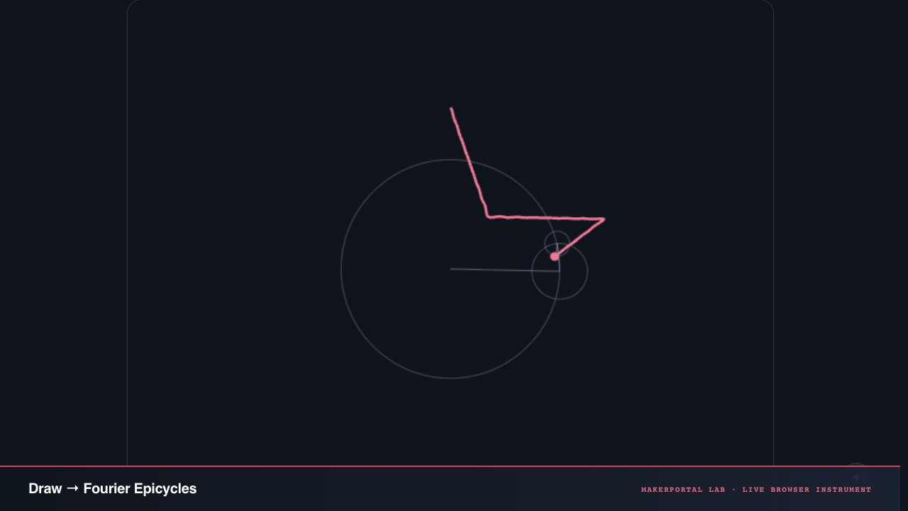
Draw a closed shape with your mouse or finger. It gets decomposed into rotating circles — a discrete Fourier series — that chain together to trace your exact path back.
Independent research instrument — not claimed as MakerPortal shipped product code. Methods, equations, assumptions, and limitations are disclosed so you can inspect what the page does and does not establish.
Draw and watch
Draw a closed shape below — a star, a loop, your initial. Let go to see it decomposed.
Anatomy of the instrument
Every pixel above answers to the math below. Here is what each piece of the canvas, the presets, the slider, and the reconstruction is actually doing — and why it is built that way.
The epicycle canvas
- 01
The coordinate mapping. The canvas is the complex plane. Every point you draw is treated as . The left edge maps to negative real values, the right edge to positive real values, and the Y-axis is the imaginary axis. This is not just a coordinate trick — it is what makes rotation become multiplication by with zero matrix overhead.
- 02
Epicycle circles and arms. Each term draws a faint circle of radius centered at the previous term's tip, plus a radial arm from that center to its own tip. Circles smaller than 1.5 px are skipped visually but still contribute to position. The arms chain tip-to-tail in amplitude-sorted order — largest first — so you see the structure emerge from the biggest contributors down to the fine detail.
- 03
How a drawing becomes a path. Mouse or touch events collect raw screen coordinates on
pointerdown/pointermove/pointerup. The raw polyline is resampled to uniformly arc-length-spaced points viaresamplePath, erasing drawing speed. The path is then treated as closed: the last point connects back to the first via modulo indexing. That closure edge is the only synthetic geometry — everything else is your hand. - 04
The terms slider. Maps from 1 to . At you see only the centroid (the DC term, which does not spin — it is the average position). Each step adds the next-largest circle. The slider is disabled until a path is finalized. Changing it clears the trail to avoid mixing reconstructions from different term counts.
- 05
The render loop. There is no numerical integration and no differential equation. Each frame computes , steps through terms computing and , pushes the final into a 420-point trail buffer, and draws. Pure trigonometric reconstruction — the epicycles are the formula, not a simulation of the formula.
The DFT — what runs when you lift the pen
This is the naive DFT — two nested loops, no FFT. Each is divided by before storage, so is already the circle radius. The frequency mapping assigns to positive (counter-clockwise) and to (clockwise). Both directions are needed for non-circular shapes.
Controls, presets, and reconstruction
- 01
The presets. Six hardcoded paths: a circle (pure ), a 5-point star (spikes at ), a lemniscate (needs balanced and ), a parametric heart, a logarithmic spiral (closed by a return line to center), and an MP monogram (multiple straight segments — Fourier hates straight lines). Each preset exercises a different spectral property.
- 02
The DFT algorithm. naive DFT — two nested loops, no FFT. For each frequency , the inner loop accumulates and with , then divides by . At , that's ~19,600 complex multiply-adds — instant in JS, and clearer to read than importing an FFT library.
- 03
Term sorting by amplitude. After computing all , the array is sorted descending by . This means the slider peels away importance rather than arbitrary high frequency. For a star, outranks despite being higher frequency — symmetry demands it. You see structure emerge, not noise. This is perceptual low-pass filtering, not classical frequency-cutoff low-pass.
- 04
Centroid subtraction. Before the DFT, the mean is subtracted from every point. This zeroes the DC component so the animation origin sits at the shape's center instead of at some canvas corner. Without this, the term would dominate with an enormous radius to the page corner, and everything else would be a tiny orbiting detail.
- 05
Path resampling and frequency mapping. The raw polyline is resampled to uniform arc-length points via
resamplePath— a linear walk along each segment at constant step size. This erases drawing speed and leaves only geometry. The frequency mapping converts standard DFT ordering (which packs positive frequencies in the first half and negative in the second) into signed integers: positive = counter-clockwise, negative = clockwise. Both directions are essential — a figure-8 needs and with near-equal amplitude.
Gear behind this build
DSP lab stack · 37 picks
Audio DSP tools37
$229.00Audio interfaceBehringer UMC1820 Audiophile 18x20 USB Audio/MIDI Interface with Midas Mic Preamplifiers and ADAT I/O | For Recording Microphones and Instruments
Audio interface used building Biquadia — 8-preamp USB I/O for real-time DSP testing.
$9.99AudioComimark 1Pcs ADMP401 MEMS Microphone Breakout Module Board for Arduino Universal 1.3cm*1cm
MEMS mic breakout used for real-time DSP experiments feeding into Biquadia.
$113.29BookAntenna Theory: Analysis and Design
Derives array factor AF=∑I_n exp(jn(kd cosθ+β)) and microstrip patch cavity model with fringing fields this sandbox implements for beam tilt and radiation efficiency.
$159.00HeadphonesAudio-Technica ATH-M50X Professional Studio Monitor Headphones, Black, Professional Grade, Critically Acclaimed, with Detachable Cable
Reference monitoring headphones used for akous's binaural audio testing.
$180.00MicrophoneBit Trade One BIMIMI - Binaural Stereo Microphone Easy BINAURAL Recording/ASMR/Podcast/Recording/Streaming / W7.2×H1.9×D2.6 inches/ADBMM
Binaural stereo mic capturing HRTF — the spatial cues this head-tracked panner approximates via ITD/ILD and quaternion yaw driving StereoPannerNode.
$56.49MicrophoneBlue Yeti Nano Premium USB Microphone - Shadow Grey (Renewed)
Compact USB condenser mic used for nymic testing.
$116.92BookComplex Analysis
Defines analytic functions, Cauchy-Riemann ∂u/∂x = ∂v/∂y, and conformal property — drag f(z)=z² and watch CR fail/preserve angles live as Ahlfors proves.
$92.40BookDigital Signal Processing
Chapter on biquad Direct Form II transposed and pole-zero placement — move poles in pole-zero explorer and hear Q/ω0 map to ring frequency as Proakis derives.
$33.86BookHigh Speed Digital Design: A Handbook of Black Magic (Prentice Hall Modern Semiconductor Design)
Defines Hammerstad-Jensen Z0, skin depth delta=sqrt(2/ωμσ), and crosstalk K_b backward coupling — closed-form behind this lab's per-unit-length L,C extraction and NEXT/FEXT formulas.
$12.69DiagnosticHiLetgo USB Logic Analyzer Device with EMI Ferrite Ring USB Cable 24MHz 8CH 24MHz 8 Channel UART IIC SPI Debug
Budget 8-ch USB logic analyzer (sigrok/PulseView). Useful for RTOS GPIO timing and SI digital demos — not a Saleae substitute in bandwidth.
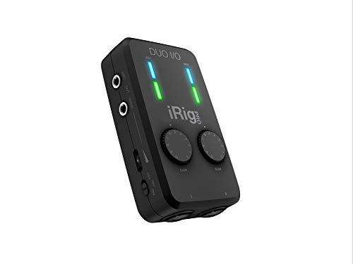
$229.99Audio interfaceIK Multimedia iRig Pro Duo I/O USB audio interface, TRS balanced & headphones outputs, audio mixer to 24-bit, midi interface for music studio, recording, podcasting, streaming & social apps
Portable 2-channel USB-C audio interface used for mobile Biquadia field recording.
$39.95BookLoudspeaker Design Cookbook
Breakup modes, cone edge termination, and waveguide directivity index — chapters 7-9 explain the cone-breakup visualization and waveguide polar math this lab implements.
$198.00BookMicrowave Engineering
Derives S-parameter conversion Z=Z0(I+S)(I-S)^-1, Smith Chart mapping Γ=(Z-Z0)/(Z+Z0), and stub matching l=λ/2π arctan(B/Y0) this bench solves continuously during drag.
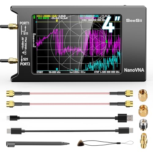
$89.99DiagnosticSEESII Upgraded NanoVNA-H4 Vector Network Analyzer, Latest V4.4 9KHz-1.5GHz HF VHF UHF 4" Touch Screen VNA Antenna Analyzer Measures S Parameters,Voltage Standing Wave Ratio, Phase,Delay, Smith Chart
Handheld VNA with touchscreen + SOL kit — S11/S21 lab companion for RF Bench and Antenna Sandbox.
$71.99KitFNIRSI 2C23T 3 in 1 Handheld Oscilloscope Multimeter DDS Generator, 2 Channels, 10MHz Bandwidth, 50MSa/s Sampling Rate, 10000 Counts, Voltage, Current, Capacitor, Resistor, Diode Test
Feed a square wave into your scope and see its Fourier epicycles live — same harmonic decomposition (odd k only) this page animates as rotating vectors.
$38.32BookRF Circuit Design
L-network matching Q = sqrt(Rp/Rs-1) and component X = ±Q*Rs formulas — this bench's auto-match button solves these analytically then animates Smith Chart journey through series L then shunt C.
$157.00MicrophoneRØDE NT-USB+ Professional-Grade USB Condenser Microphone For Recording Studio Quality Audio Directly To A Computer Or Mobile Device, Black
USB condenser mic used for nymic testing.
SensorRTL-SDR Blog V4 R828D RTL2832U 1PPM TCXO HF Bias Tee SMA Software Defined Radio with Dipole Antenna Kit
100kHz-1.75GHz low-cost SDR for passively listening to patch array sweeps — compare simulator's beam steering phase Δφ = kd sinθ with over-the-air measured phase progression across 2.4GHz.
$43.68BookThe Scientist & Engineer's Guide to Digital Signal Processing
Intuitive pole-zero explanation — why a pole near unit circle rings, zero near kills — the exact intuition this pole-zero explorer makes tangible with drag-to-listen.
$299.99MicrophoneSennheiser Pro Audio Sennheiser Pro Audio Wireless Microphone System, Black (MKE600)
Wireless mic system used for akous's ambient/binaural field recording.
$23.80MicrocontrollerTeensy 4.0
600 MHz Cortex-M7 — high-rate control loops and DSP on the RTOS / FOC benches. Carried by SparkFun (third-party PJRC; tracked referral).
$319.00MicrophoneShure MV7+ Podcast Dynamic Microphone with Stand – OBS Certified, Enhanced Audio, LED Panel, USB-C & XLR Outputs, Auto Level Mode, Digital Pop Filter – for Podcasting, Streaming, and Recording, Black
USB/XLR hybrid mic used building and testing nymic.
$237.00MicrophoneShure MV88+ Video Kit Digital Stereo Condenser Microphone for iPhone, Android, Mac & PC - Portable Recording Mic with DSP Controls, Headphone Monitoring & Tripod, Black
Portable stereo condenser mic kit used for Biquadia field/video capture.
$275.45BookSignals and Systems (Prentice-hall Signal Processing Series)
Defines the DTFT, DFT, and complex Fourier coefficients c_k this visualizer computes — chapters 3-5 derive the exact reconstruction formula tracing your doodle.
$13.90KitAURSINC SMA Calibration Kit and SMA Male to Male Jumper for NanoVNA H H4 F V2 V3 SAA Mini1300 PS100 Vector Network Analyzer Antenna Analyzer
SOL cal standards + SMA jumper for NanoVNA H/H4 — SI Lab and RF Bench SOLT demos.
$113.00HeadphonesSony MDR7506 Professional Large Diaphragm Headphone
Reference studio headphones used for akous's binaural audio testing.
$71.89BookImmersive Sound: The Art and Science of Binaural and Multi-Channel Audio (Audio Engineering Society Presents)
Derives HRTF, ITD = d/c sinθ, and head-tracking compensation — the exact panning law this playground interpolates as you drag yaw.
$26.80MicrocontrollerTeensy 4.0 (Headers)
600 MHz M7 — flash the DF2T biquad cascade from Biquadia’s DSP core (pair with the Rev D audio shield for codec I/O) and hear the same filter your design exports here.
$206.99DiagnosticAURSINC TinySA Ultra+ ZS406 Spectrum Analyzer with 50W N-Type 50dB RF Attenuator, 100kHz-5.4GHz, 4.0" Touchscreen HW V0.4.6, 2-in-1 Signal Generator, DC-3GHz 50Ω Ham Radio Test Kit
Portable spectrum analyzer + attenuator kit — EMI and spur checks next to the RF Bench.
$139.98MicrophoneminiDSP UMIK-1 USB Measurement Calibrated Microphone
Calibrated USB mic with individual cal file — measure your room's RT60 and modal peaks to validate the room-mode eigenfrequencies this calculator predicts.
$95.34BookUnderstanding Digital Signal Processing
Chapter on DFT and windowing explains spectral leakage and Gibbs phenomenon visible as overshoot when you draw sharp corners in the epicycles tracer.
$8.99AudioSABRENT USB External Stereo Sound Adapter for Windows and Mac. Plug and Play No Drivers Needed. (AU-MMSA)
USB audio interface used in early Biquadia MEMS-mic prototyping.
$54.49BookVisual Complex Analysis: 25th Anniversary Edition
Entire premise is epicycles-as-complex-exponentials — e^{iwt} spinning phasors whose sum is a discrete Fourier series, same DFT this playground draws with.
$31.63BookVisual Differential Geometry and Forms: A Mathematical Drama in Five Acts
Sequel to Visual Complex Analysis — explains how conformal warp preserves infinitesimal circles, which you see as grid squares stay square under holomorphic f(z).
$105MicrophoneminiDSP UMA-8 USB Microphone Array
7-element MEMS microphone array with onboard XMOS DSP for raw channel output and real-time spatial audio / beamforming research.
$315.06HeadphonesSennheiser HD 650 Open-Back Headphones
300-ohm audiophile reference open-back headphones used for binaural dummy head calibration and earphone transfer function measurements.
$530ApparatusSR3D® Dummy Head MKIII
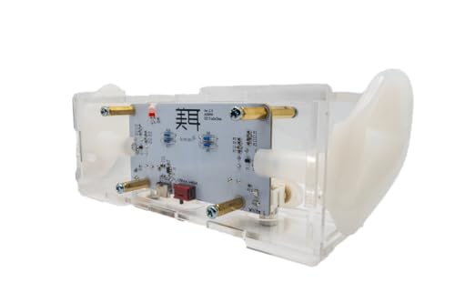
Binaural dummy head acoustic fixture with anatomical silicone pinnae and Primo EM272 electret capsules for HRTF and headphone measurement.
Prices shown were retrieved from the Amazon Product Advertising API on 19 July 2026 and are indicative only — the price and availability on Amazon at the time of purchase apply.
Prices shown were checked against the Amazon product listing on 9 August 2026 and are indicative only — the price and availability on Amazon at the time of purchase apply.
More gear across every app: the full Gear list →
Essence
Any doodle is just circles spinning at the right speeds.
Draw a star, a heart, a shaky signature. Once you lift the pen, the path doesn't look like a single messy line anymore — it becomes a machine built from pure circular motion, one circle riding on the tip of another, all spinning at integer multiples of a base rate, reconstructing your exact wobble.
Ptolemy tried this to explain planets, stacking epicycles upon epicycles to fit retrograde loops. Fourier proved you can do it perfectly for any closed curve. Same math that powers spectral analysis in Biquadia, just rotated 90 degrees in your mind: instead of decomposing sound pressure over time into sine waves, you decompose and over time into spinning complex exponentials.
This playground makes that literal. You give it , a walk in the complex plane. It computes how much of each pure spin you need, then plays them back tip-to-tail. The tip draws you.
The intuition — ink as complex numbers
The canvas is the complex plane. Each point you draw is . Why complex? Because rotation becomes multiplication. Multiply by and you rotate by with no matrix, no bookkeeping. A pure circle at constant speed is just — radius , frequency , starting angle .
Your drawing is a loop with from 0 to 1. Fourier's trick: any such loop, no matter how jagged, is a sum of circles spinning at integer rates . doesn't spin — it's the centroid, the average position. goes once around during your loop. goes once the other way. twice as fast, and so on.
Magnitude controls size. If coefficient has large , its circle is big and carries most of the shape. Phase controls orientation — where the circle starts at . Add all circles tip-to-tail and the final tip traces exactly. Remove small circles and you still get the gist but lose fine jitter. That is low-pass filtering.
Three details make this playground feel right:
- Resampling to 140 points. Your hand produces uneven spacing — fast strokes leave few samples, slow strokes leave many. The code walks the polyline by arc length and emits uniformly spaced points via resamplePath. That erases drawing speed and keeps only geometry. Constant keeps the DFT at cheap and the animation crisp.
- Centroid first. Mean is subtracted before transform, computed as . The animation origin is that . Without this, the term would dominate with a huge radius to the page corner, and everything else would be a tiny detail orbiting far away.
- Sorted by amplitude. Raw frequency order is . Visually more useful: sort by , biggest radius first. Then slider peels away importance rather than arbitrary high frequency. You see structure emerge, not noise.
Animation runs ms per cycle — sweeps every nine seconds, slow enough to see each epicycle turn. The pink trail buffer holds points, about three full loops of history, then overwrites. That persistence lets you compare reconstruction vs ideal without infinite ink.
Think like this
A circle of radius spinning at turns per loop and offset by is . Chain 60 of them: first circle's tip becomes second's center. Biggest first. That's all this page does.
Radius and phase decoded
radius
start angle
turns per loop, negative = clockwise
In code each term stores re, im, freq, amp, phase. is already divided by , .
Why uniform resample matters
If you kept raw mouse samples, fast strokes would be underweighted. Arc-length parameterization makes geometric, not temporal. 140 points captures a 5-point star's 10 corners easily, yet keeps DFT at complex multiply-adds — instant in JS.
The math — DFT to epicycles, no black boxes
1. From stroke to signal
After resampling you have points , , closed so . Build . Subtract centroid to place animation origin at shape center. Call the zero-mean signal .
2. Analysis — Discrete Fourier Transform
DFT asks: how much of each pure spin lives inside ? Project onto each spin:
Code loops exactly this: , with , then . So stored re,im already include 1/N.
Interpretation: is amplitude and phase of the circle that spins times per loop. In raw DFT ordering, corresponds to negative frequency , i.e., clockwise spins. The code converts: freq = k <= N/2 ? k : k-N. That's why you see both positive and negative freq in sorted terms — you need both directions to make non-circular shapes.
3. Synthesis — epicycle reconstruction
Rebuild the path at continuous time by summing circles:
In animation , . Each frame computes , steps , tip-to-tail. Trail pushes final (x,y).
Use terms instead of and you get low-pass filtering. Dropping high |k| removes fast wobble — exactly how JPEG discards high DCT coefficients, how audio codecs shave brilliance, how Biquadia's filter shelves high frequencies. Keeping only biggest rather than lowest |k| is even smarter: biggest circles first, perceptually optimal compression.
Sharp corners need high |k|. Truncate and you see Gibbs phenomenon: ringing overshoot near discontinuities, about overshoot that never vanishes, only compresses in width as you add terms. That's why a star point looks rounded with few terms, then develops a tiny ripple that hugs the tip as you crank to 60.
State that actually travels
140 complex coefficients, DC removed for origin. Sorted view keeps of them. Slider maps to visual fidelity. No FFT — naive DFT, 19.6k ops, faster to write than to import FFT and clearer to read.
Frequency mapping
counter-clockwise, clockwise. Need both to trace arbitrary loops. A perfect circle needs only (or -1). A figure-8 needs balanced.
Low-pass as smoothing
Energy compaction: usually top 8 circles hold of power for cartoon shapes. Rest is edges, hand tremor, sampling noise. Slider is literally a bandwidth knob.
Why Gibbs rings
A sharp corner is high-frequency. Truncate Fourier series and partial sum overshoots by . Add more terms: overshoot moves closer to corner, doesn't vanish. Draw a star and push slider — watch tips ripple, that's Gibbs live.
Playbook — what to draw, what the slider means
Start with presets
Circle: one dominant circle, others near zero. Slider jumps from dot at centroid to perfect circle. Pure tone in audio terms.
Star: 5 points = 5-fold symmetry. Spectrum spikes at . With 5-8 terms you get lumpy star; 15+ sharpens points but Gibbs ripples appear at tips. Shows why high |k| equals edge detail.
Infinity / figure-8: needs and with almost equal amplitude — counter and clockwise battles. Two terms give an ellipse, three give a pinched loop. Nice demonstration that you can't make a figure-8 from only CCW circles.
Heart: smooth bulge plus sharp cusp at bottom. Low capture bulge, cusp needs high . Watch bottom point evolve: rounded, pointed, slight ringing either side.
Spiral: not closed, but code closes it with a line back to center. That closure edge is a discontinuity, so spectrum spreads wide — needs many terms, low-pass looks like shrinking coil. Good stress test for Gibbs.
MP monogram: multiple straight segments + bowl. Fourier hates straight lines and corners — needs many high frequencies. Demonstrates compression limit: text is hard.
The terms slider decoded
— dot at centroid . You removed all rotation, left only DC. Slightly anticlimactic, proves DC handling works.
to 3 — best-fit ellipse(s). Two largest circles make an ellipse, third adds offset bulge. Any smooth loop looks roughly elliptical at this level — same reason first two principal components capture most variance.
to 10 — recognizable. Star shows 5 points, heart shows asymmetry, infinity pinches. This band is sweet spot for "aha" — enough structure, not too much clutter.
to 30 — details, corners start to bite. You trade cleanliness for fidelity. Good range to see Gibbs begin.
to 60 — nearly pixel-perfect, includes hand tremor and resampling artifacts. At 60 you kept of coefficients — close to lossless. Beyond 60 diminishing returns; remaining terms are near noise floor.
Draw your own — tips
- Draw slowly and close the loop near start — closure gap is linearly interpolated and creates a high-frequency edge.
- Single non-intersecting loop beats scribble. Self-intersections still work, but spectrum smears — more high |k| needed.
- If you want clean circles, keep it convex. If you want ringing, draw sharp zig-zag — that's Gibbs you can trigger on demand.
- Loop time is fixed for perception, not tied to draw speed. That decoupling is deliberate — geometry, not timing.
Tweaks that matter
Uniform arc-length resample, walk. 140 balances detail vs cost and visual clutter. Raise it and you get hairline fidelity but slider needs more terms; lower and sharp corners alias.
ms
Full period for wrap. Chosen so circle completes 10 turns in 9 s — you can still follow it by eye. Faster would blur, slower would drag. Trail = 3 loops covers persistence without unbounded memory.
Sorting by amp not |k|
Low |k| first would give classic low-pass. Sorting by gives perceptual low-pass — biggest visual contributors first. For star, outranks despite higher frequency, because symmetry demands it.
Honesty — what is real
DFT formula exact, implemented as double loop matching textbook definition, no FFT trickery. Centroid computed as mean then subtracted — origin is true DC. Complex exponentials use cos/sin via Math.hypot/atan2 for phase. Magnitude and phase decode directly to radius and start angle — no hidden scaling. Sorting stable and deterministic.
Honesty — what it simplifies
Resampling erases time — your fast vs slow strokes become equal length. Closure forced by modulo wrap: last point to first via straight line, even if you left a gap. No windowing, no pre-filter, so sharp closure edge leaks high frequency. Uniform sampling not perceptually weighted. Canvas is float32 raster, not analytic curve — trail anti-aliased by browser. O(N²) DFT doesn't scale to thousands of points, but we never go there. Trail is approximate history, cleared on slider change to avoid mixing reconstructions.
Why this matters for audio DSP
Same transform, different domain. Biquadia's spectrogram shows sliding over windows of audio. Here is not time but position along loop. Sorting by amp is like finding dominant harmonics — fundamental vs overtones. Low-pass by dropping high |k| is identical to low-pass filter in audio: it smooths transients, causes pre-ring near attacks, which is Gibbs in time domain. Once you see it on a star, you'll hear it on a snare.
Two gotchas worth knowing
N=140 limits the capture fidelity
With sample points the Nyquist limit is . Any shape feature finer than about of the loop perimeter is undersampled and will alias into lower frequencies — sharp corners, rapid zig-zags, or hand tremor faster than that spatial bandwidth. Shapes drawn in a single quick flick with few mouse samples will be coarsely interpolated. The resampling also erases your stroke speed, which is usually desirable but means fast-sketched detail is lost. Try the MP preset at : the straight vertical strokes of the letters never fully sharpen because N=140 cannot encode a true step.
DFT vs. continuous Fourier series
This page uses a discrete Fourier transform on 140 samples, not the continuous Fourier integral . The DFT implicitly assumes your signal is periodic with period — that's why the path is forced closed. If you draw a spiral that doesn't naturally close, the straight-line closure edge injects a broadband discontinuity whose high-frequency energy spreads across many terms. A continuous Fourier series of a truly smooth closed curve would have exponentially decaying coefficients; the DFT gives you polynomial decay at best, limited by the sampling resolution. Also, the DFT lacks windowing: the hard closure acts like a rectangular window, causing spectral leakage that shows up as noise in the smaller terms.
If you want to see the same transform applied to actual audio signals — same math, different domain — read the Biquadia internals: the Biquadia deep-dive →
JavaScript, the DFT and reconstruction
These functions run in every browser on this page. The DFT is a textbook double-loop — no FFT, no libraries. Drop it into any canvas project. If you are feeding real-time audio through an audio interface, the same logic ports directly to C or Python for live spectral analysis.
DFT + epicycle reconstruction
function computeDFT(points) {
const N = points.length;
const cx = points.reduce((s, p) => s + p.x, 0) / N;
const cy = points.reduce((s, p) => s + p.y, 0) / N;
const signal = points.map(p => ({ re: p.x - cx, im: p.y - cy }));
const terms = [];
for (let k = 0; k < N; k++) {
let re = 0, im = 0;
for (let n = 0; n < N; n++) {
const phi = (2 * Math.PI * k * n) / N;
re += signal[n].re * Math.cos(phi) + signal[n].im * Math.sin(phi);
im += -signal[n].re * Math.sin(phi) + signal[n].im * Math.cos(phi);
}
re /= N; im /= N;
const freq = k <= N / 2 ? k : k - N;
terms.push({ re, im, freq,
amp: Math.hypot(re, im),
phase: Math.atan2(im, re) });
}
terms.sort((a, b) => b.amp - a.amp);
return { terms, centroid: { x: cx, y: cy } };
}
function reconstruct(terms, centroid, t, M) {
let x = centroid.x, y = centroid.y;
for (let i = 0; i < M; i++) {
const { freq, amp, phase } = terms[i];
const ang = 2 * Math.PI * freq * t + phase;
x += amp * Math.cos(ang);
y += amp * Math.sin(ang);
}
return { x, y };
}Frequently asked questions
What is a DFT and how does it decompose a drawing?
The Discrete Fourier Transform (DFT) asks: how much of each pure spin e^(i·2π·k·n/N) lives inside your signal? It takes your N sample points as a complex signal z_n = x_n + i·y_n and projects them onto N complex exponentials — one for each integer frequency k. Each output X_k is a complex number whose magnitude tells you the radius of a circle spinning k times per loop, and whose angle tells you where that circle starts. The shape is literally the sum of those circles drawn tip-to-tail.
What are epicycles and why do they trace any closed shape?
An epicycle is a circle whose center rides on the circumference of another circle. Ptolemy stacked them to model planetary retrograde motion centuries before calculus existed. Fourier proved mathematically that any closed curve — no matter how jagged — can be expressed as an infinite sum of circles spinning at integer multiples of a base frequency. The playground computes a finite approximation using N=140 terms: the largest circles carry the overall silhouette, and the smallest circles add fine detail. The final tip of the last circle is exactly one point on the reconstructed path.
How does the Fourier series relate to this epicycle visualization?
A Fourier series represents a periodic function as a sum of sines and cosines. The epicycle visualization is the same idea rotated into the complex plane: each term X_k·e^(i·2π·k·t) is a circle of radius |X_k| rotating at frequency k. The real part gives x(t), the imaginary part gives y(t). So your drawing on the 2D canvas is literally a periodic complex-valued function z(t) = x(t) + i·y(t), and the DFT gives you its Fourier coefficients. It is the exact same math as a spectrogram, just with the time axis traded for position along the curve.
Why does N=140 limit the capture fidelity? What is the Nyquist limit here?
With N=140 sample points, the highest frequency you can represent without aliasing is k = N/2 = 70 (the Nyquist frequency). Any shape detail smaller than about 1/70 of the loop is undersampled — sharp corners, tight zig-zags, or hand tremor faster than that spatial frequency will alias into lower frequencies. The resampling to 140 uniform arc-length points also erases your drawing speed: fast strokes and slow strokes become equally dense along the path, so only the geometry matters. Shapes with features finer than ~1/140 of the total arc length will be blurred or lost.
How does signal reconstruction work from DFT coefficients back to the drawing?
Reconstruction is the synthesis step: start at the centroid, add the largest circle first (its tip becomes the center of the next), then chain circles tip-to-tail in amplitude-sorted order. At any time t between 0 and 1, each term contributes r_k·cos(2π·f_k·t + φ_k) to x and r_k·sin(2π·f_k·t + φ_k) to y. The final (x, y) is a point on the reconstructed curve. Using all N terms gives you the exact input shape back. Using fewer terms — controlled by the slider — is low-pass filtering: you drop the smallest, fastest circles and get a smoothed approximation. This is the same principle behind JPEG compression (dropping high DCT coefficients) and MP3 encoding (dropping inaudible high frequencies).
Shareable still
The instrument, captured—not illustrated.
This 16:9 frame is rendered from the real browser instrument above. It is the page's canonical preview for image search, link unfurls, and posts that need to show what the tool actually does.
Download 1280 × 720 JPEG
Continue the experiment