Playground · research instrument

DSP · Audio

Room Mode Calculator

Enter your room dimensions and see every standing-wave resonance up to a chosen frequency. Identify which modes pile up at your listening position, and explore the pressure pattern of any single eigenmode across the floor plan.

Independent research instrument — not claimed as MakerPortal shipped product code. Methods, equations, assumptions, and limitations are disclosed so you can inspect what the page does and does not establish.

Standard room size? 653 rooms are already solved — modes, pile-ups and proportions, no input needed.

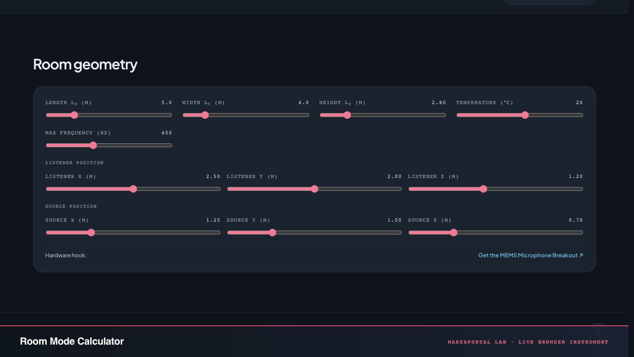
Browse solved rooms →

Room geometry

Length L_x (m)5.0Width L_y (m)4.0Height L_z (m)2.8Temperature (°C)20Max frequency (Hz)400

Listener position

Listener X (m)2.50Listener Y (m)2.00Listener Z (m)1.20

Source position

Source X (m)1.25Source Y (m)1.00Source Z (m)0.70

Hardware hook:Get the MEMS Microphone Breakout ↗

Results

Room metrics

Volume: 56.0 m³
Surface area: 90.4 m²
Edge length: 47.2 m
Speed of sound: 343 m/s
Schroeder f_c: —
Total modes: 0

Mode counts

Axial: 0
Tangential: 0
Oblique: 0
Density at f_max: 3.28 /Hz

Modal frequency table

#	n_x	n_y	n_z	f (Hz)	Type	Pressure at listener

2D Pressure map

Horizontal slice at listener height (z = 1.20 m). Each cell's colour shows the standing‑wave pressure of the selected mode.

Mode to displayGrid res40

Pressure map—

Essence

Your room is a 3D guitar string you didn't pluck — but bass does.

Clap in an empty box and some notes keep singing. Not echo — resonance. Air trapped between parallel walls behaves exactly like a string pinned at both ends: only wavelengths that fit an integer number of half-waves survive. In 1D that's $f=n c/2L$ . In 3D it's the same idea three times — combine half-waves along length, width, and height, and you get a grid of allowed tones. Those are room modes. Everything that booms, drones, or disappears when you move the couch lives here.

The ghost in the calculator is the assumption that walls are brick-ideal — perfectly rigid, zero absorption. Real walls breathe, flex, soak energy, shift peaks down a few Hz and smear them. Yet the rigid ideal predicts measured axial frequencies within 2–5% in concrete rooms and tells you where to put a sub to excite or avoid a mode — because nodes are geometry, not damping.

1. From wave equation to cosine lattice

Start with wave equation $\nabla^2 p = (1/c^2)\partial^2 p/\partial t^2$ . Seek separable harmonic solution $p(x,y,z,t)=X(x)Y(y)Z(z)e^{j\omega t}$ . Neumann walls — particle velocity zero normal to wall — mean $\partial p/\partial n =0$ at $x=0,L_x$ etc.

That boundary condition quantizes wavenumbers: $k_x = n_x \pi/L_x$ , $k_y = n_y \pi/L_y$ , $k_z = n_z \pi/L_z$ with $n_x,n_y,n_z\in\mathbb{N}_0$ not all zero. Total $|\mathbf{k}| = \sqrt{k_x^2+k_y^2+k_z^2} = \omega/c$ . Divide by $2\pi$ :

f_{n_x,n_y,n_z} = \frac{c}{2} \sqrt{\left(\frac{n_x}{L_x}\right)^2 + \left(\frac{n_y}{L_y}\right)^2 + \left(\frac{n_z}{L_z}\right)^2}

$c$ itself comes from temperature: $c(T)=331.3\sqrt{1+T/273.15}$ m/s. So a hot room tunes modes up ~0.17% per °C — 0.6 Hz shift at 100 Hz per 3 °C. Measurable. The calculator recomputes it live.

2. Pressure shape — where sub and ears couple

For rigid walls the eigenfunction is pure cosines product:

p_{n_x n_y n_z}(x,y,z)=\cos\left(\frac{n_x\pi x}{L_x}\right)\cos\left(\frac{n_y\pi y}{L_y}\right)\cos\left(\frac{n_z\pi z}{L_z}\right)

Value in [-1,1]. Antinode ±1 at every wall — pressure maximal, velocity zero. Node 0 where $n_x\pi x/L_x = \pi/2, 3\pi/2$ ... i.e. $x = L_x/(2n_x), 3L_x/(2n_x)$ ... That's a plane. Two cosines zero → nodal line. Three → nodal point.

Coupling is ruthlessly simple: mode amplitude $\propto p(\text{source})\times p(\text{listener})$ . Put a sub at a pressure antinode (wall) and it maximally drives that mode. Put it at a node and that mode goes silent — even though other modes still fire because their nodes are elsewhere. Same at listener: at a node you don't hear that mode, even if source excites it. This is why corner placement (all cos=±1) excites every mode, and why moving a sub 70 cm can kill a 40 Hz boom without EQ.

Velocity is 90° out of phase spatially: $\mathbf{v}\propto \nabla p$ . Where $p=0$ , particle velocity peaks — good place for porous absorbers which need air motion. Where $p=±1$ , velocity zero — absorbers do nothing, but membrane traps work.

3. Why modes look like they do on the map

The 2D slice fixes $z = z_{listener}$ and shows $p(x,y,z)$ . Red/blue are ± pressure. Watch (1,0,0): left red, right blue, one half-wave across length. (2,0,0): red-blue-red — two half-waves. (1,1,0): checkerboard — one wave along x and y, hitting four walls. Higher indices tile faster, density $\propto f^2$ .

The listener diamond and source dot on the map are not decoration — the table's "Pressure at listener" column is exactly $p(x_L,y_L,z_L)$ and source coupling would be $p(x_S,y_S,z_S)$ . Scan the table: if a mode is +0.99 at listener, that frequency will dominate at the chair; -0.03 means you're sitting in its null.

Axial / Tangential / Oblique — why energy differs

Axial $(n_x,0,0)$ — one index non-zero. Wave bounces between two parallel walls only. Two reflections per cycle, minimal wall contact, highest Q, biggest peak. (1,0,0) at $c/2L_x$ is almost always the worst offender.

Tangential $(n_x,n_y,0)$ — two non-zero. Four walls per cycle. Energy hits walls more often, losses double ~ — about 3 dB less energy than axial after averaging.

Oblique $(n_x,n_y,n_z)$ — three non-zero. All six surfaces. Least energy in practice, ~6 dB below axial, but most numerous: number of oblique grows as $f^3$ . Topology: 1-0-0 is plane wave, 1-1-0 is diagonal, 1-1-1 bounces around room like a billiard.

Real rooms weight axials strongest, which is why your table highlights axial rows — they need treatment first.

Schroeder / Schroeder-Bay — when statistics beats determinism

f_c = 2000 \sqrt{\frac{T_{60}}{V}}

$T_{60}$ here is estimated from Sabine 0.161 V/A with $\bar{\alpha}=0.15$ typical furnished. $f_c$ is where 10 modes overlap within a mode's half-power bandwidth — above it, individual peaks blur into a statistical tail. Below, you hear discrete colouration. Rule of thumb: $V$ in m³, $T_{60}$ in s. 60 m³ living room, 0.4 s → $f_c\approx 163$ Hz. That's why bass below ~200 Hz needs modal fixes (placement, traps, EQ), above it needs absorption/diffusion — different physics. Constant 2000 varies by school (1500–4000); we use 2000 as conventional. Bonello's extra check: modal density should monotonically increase in each third-octave — if not, ratios are poor. Sepmeyer and Louden suggested $L_x:L_y:L_z \approx 1:1.6:2.33$ or 1:1.4:1.9 to spread axials. Use this tool to test any ratio — look for piled axial pairs within 5 Hz, those will ring.

Nodal placement as acoustical judo

Want less (2,0,0)? Place sub at $x=L_x/4$ or $3L_x/4$ because $\cos(2\pi x/L_x)=0$ there. Want fewer nulls at listening spot? Avoid listener at $x=L_x/2$ for (1,0,0) (null at center), avoid $y=L_y/2$ for (0,1,0), etc. The map makes this visual: drag source or listener in your head to a white (zero) region for the bad mode.

Full elimination impossible because nodes differ per mode. Trick: sub at 1/3 length excites (1,0,0) and (2,0,0) moderately but nulls (3,0,0). Two subs at 1/4 and 3/4 cancel even axials via destructive pressure summation — principle behind double-bass arrays and CABS.

For porous absorption: put it where $\nabla p$ maximal (nodes) and thick enough $> \lambda/10$ or spaced off wall. For pressure traps (membrane): put at antinodes (walls).

What ideal model ignores

Finite wall impedance → eigenfrequencies shift down 2–5% and Q finite (~10–40 at low end). Damping not modal-independent: tangential/oblique damp faster because more wall hits.

Coupling: real modes are not orthogonal with lossy walls; energy leaks between them. Non-rectangular (L-shaped, vaulted) splits degeneracy — our integer triple no longer holds. Furniture acts as scatterer, adds absorption $\approx$ area·α and breaks perfect cosine via diffusion.

Air absorption above 2 kHz in large rooms matters (Sabine's 4mV term). The pressure map shows undamped $p$ , not SPL re energy — it's geometric ideal, not FEM.

Playbook — tame the booms

1. Find the offender

Enter $L_x$ , $L_y$ , $L_z$ . Set max freq 300 Hz — bass region. Sort by freq: lowest three axials are your enemies. Note where two axials land within 4 Hz — Bonello violation, audible double peak. Example 5×4×2.8 m: $(1,0,0)=34.3$ Hz, $(0,1,0)=42.9$ Hz, $(0,0,1)=61.3$ Hz. Those three define your room's signature.

2. Use the map to move intelligenty

Pick mode (1,0,0) in dropdown. See red left, blue right. Drag listener (mentally) to center white line → pressure 0 → that mode disappears at ear. Pick (0,1,0), same along width. Real listening spot is compromise — stay >0.3 m from all walls, avoid exact centers L/2 if you want to hear axial at all, sit at center if you want to null it. For sub: corner = excite all, 1/2 wall = kill first axial, 1/4 wall = kill second, 1/3 and 2/3 dual subs kill even more. Check source pressure vs mode in table extension idea: source coupling = $p(x_S)$ similar to listener.

3. Ratio tune / break tie

If building or choosing room, sweep $L_x$ slider ±10 cm and watch table — aim for axial spacing >5% apart below 100 Hz and increasing density per third-octave. Louden 1:1.4:1.9, Sepmeyer 1:1.28:1.54, EBU 1:1.25:1.6 all better than cube (1:1:1 disaster). The Schroeder readout tells you where you can stop caring — above $f_c$ , use absorption, not geometry.

4. Treatment logic

Below $f_c$ : move sub/listener (free), then EQ (narrow notch -3 to -6 dB, Q 8–12) at modal frequency, then resonant traps tuned to $f_{mode}$ placed at pressure antinodes (wall). Porous panels effective only if 10–15 cm thick or spaced, placed at nodes (velocity max). Above $f_c$ : broadband absorption, aim $T_{60}\approx0.3$ –0.5 s for small rooms, calculate via $A =0.161 V/T_{60}$ . The pressure map's +1/-1 scale reminds you: porous does nothing at +1 walls.

5. Validate with measurement

Run a sine sweep at listening position — peaks in transfer function should match table within a few Hz. Nulls should match nodes. If measured peak higher Q than expected, wall is more rigid than assumed; if lower and broader, extra absorption present. Use that to update $\bar{\alpha}$ and predict $T_{60}$ .

Honest limits

Rigid-wall, undamped, rectangular, no coupling, no air absorption. Real $f_n$ lower due to wall compliance. Damping and modal overlap shift peaks. Yet axial ordering, nodal geometry, and density growth are robust — trust them for placement and ratio decisions, not for absolute SPL to 0.1 dB.

Quick reference

$p(x,y,z)=\cos\frac{n_x\pi x}{L_x}\cos\frac{n_y\pi y}{L_y}\cos\frac{n_z\pi z}{L_z}$
Coupling $\propto p_{src}\,p_{lst}$ — zero at node, max at wall.
Modal density $\propto f^2 V$ — sparse below $f_c$ , statistical above.

Anatomy of the instrument

Seven sliders, one SVG map, one live table. Here is what each control and visualization is actually doing under the hood — and why the slider limits, the color scale, and the cell resolution were chosen the way they are.

The input controls and metrics

01
Room dimensions (Lx, Ly, Lz). Range sliders with linked numeric readouts. The readParams() function pulls all values and feeds them to the roomModes() solver. Slider max values are deliberately capped (Lx/Ly 1–20 m, Lz 1–10 m) because below 1 m the modal density explodes and above 20 m you're in a hall where statistical acoustics replaces modal analysis.
02
Temperature. This sets $c(T)$ via ISO 9613-1 and feeds every frequency calculation. At -10 °C, $c \approx 325$ m/s; at 45 °C, $c \approx 358$ m/s — a 10% spread. Every mode frequency shifts proportionally. The Schroeder frequency also shifts because T₆₀ depends on $c$ through the Sabine constant 0.161.
03
Listener and source positions. Six additional range sliders whose max values update dynamically to stay within the room bounds. When you drag a room dimension slider, updateReadouts() re-clamps the listener/source max values so you can't position them outside the room. Both positions feed the pressure-at-listener column and determine the dot/diamond positions on the SVG map.
04
The metrics dashboard. Volume, surface area, and edge length are simple geometry. Schroeder frequency uses Sabine with ᾱ=0.15 — deliberately a conservative estimate because real furnished rooms typically have ᾱ between 0.12 and 0.25 at low frequencies. The mode counter runs all three types, while density at f_max evaluates the Weyl volume, surface, and edge terms to estimate how many additional modes fit in the next hertz.

The mode-counting loop

roomModes(Lx, Ly, Lz, c, fmax) iterates integer triples (nx, ny, nz) from 0 upward, computes $f = (c/2)\sqrt{(n_x/L_x)^2 + (n_y/L_y)^2 + (n_z/L_z)^2}$ , halts when f exceeds fmax, and classifies each triple as axial (one non-zero), tangential (two), or oblique (three). This is an exhaustive search, not a formula — for a 5×4×2.8 m room up to 400 Hz, it produces about 450 modes. The algorithm stops per-axis loops when a single-axis contribution alone exceeds fmax.

The pressure map and table

05
SVG pressure map. Built entirely from <rect> elements in an inline SVG — no canvas, no WebGL. Each cell computes $p(x,y,z_{listener})$ at its centroid via modePressure() which evaluates $\cos(n_x\pi x/L_x)\cos(n_y\pi y/L_y)\cos(n_z\pi z/L_z)$ . The color is HSL with hue at 0° (positive/red) or 240° (negative/blue), saturation proportional to |p|. The grid resolution slider (15–60 cells) trades visual fidelity for DOM weight.
06
Colorbar and legend. A linear gradient from −1 (blue) through 0 (white) to +1 (red), drawn as a vertical bar to the right of the map. The listener dot (white) and source dot (CTAs colored) are overlaid at their scaled xy positions. The dimension labels Lx and Ly are annotated at the bottom and left of the map, rotated for Ly.
07
The modes table. Built by mapping the sorted mode array to HTML rows, capped at 200 rows with a truncation notice. Rows are color-coded by type: green-tinted axials, yellow-tinted tangentials, purple-tinted obliques. Any mode with |p| > 0.5 at the listener position gets a left-border highlight — these are your priority targets. The table-note paragraph updates to tell you how many modes are shown vs total.
08
No idle render loop. The page computes on every slider input event — no requestAnimationFrame, no polling. The handleInput() function re-clamps listener/source positions, calls recalculate() which runs the mode solver, builds the table, populates the dropdown, and redraws the SVG. When you change the mode dropdown or grid resolution, only drawPressureMap() re-runs — the mode table is not rebuilt.

Gear for room measurement & treatment

Room acoustics stack · 22 picks

Measurement mics & monitors22

$159.00Headphones

Audio-Technica ATH-M50X Professional Studio Monitor Headphones, Black, Professional Grade, Critically Acclaimed, with Detachable Cable

Reference monitoring headphones used for akous's binaural audio testing.

DSP · Audio

$159.00 USDView ↗

$25.90Microphone

BEHRINGER ECM8000

Reference omni for acoustic measurement — captures the same pressure field these fast calculators approximate with ray-tracing and modal sums.

$25.90 USDView ↗

$229.00Audio interface

Behringer UMC1820 Audiophile 18x20 USB Audio/MIDI Interface with Midas Mic Preamplifiers and ADAT I/O | For Recording Microphones and Instruments

Audio interface used building Biquadia — 8-preamp USB I/O for real-time DSP testing.

DSP · Audio

$229.00 USDView ↗

$56.49Microphone

Blue Yeti Nano Premium USB Microphone - Shadow Grey (Renewed)

Compact USB condenser mic used for nymic testing.

DSP · Audio

$56.49 USDView ↗

$9.99Audio

Comimark 1Pcs ADMP401 MEMS Microphone Breakout Module Board for Arduino Universal 1.3cm*1cm

MEMS mic breakout used for real-time DSP experiments feeding into Biquadia.

DSP · Audio

$9.99 USDView ↗

$81.31Microphone

Dayton Audio EMM-6 Precision Omnidirectional Electret Condenser Microphone for Room Acoustic Analyzers and Audio Measurement Systems, Calibration Data File with Response Graph Included

Omni condenser with cal file — pair with REW to measure SPL, RT60, and comb filtering the acoustic calculator suite computes via image-source method.

$81.31 USDView ↗

$59.98Microphone

Dayton Audio EMM-6 Precision Omnidirectional Electret Condenser Microphone for Room Acoustic Analyzers and Audio Measurement Systems, Calibration Data File with Response Graph Included

Latest EMM-6 variant with calibration file — measure waveguide polar response and cone-breakup waterfall to validate directivity index this lab computes.

$59.98 USDView ↗

$49.98Microphone

Dayton Audio iMM-6C Calibrated Measurement USB-C Microphone for iPhone, iPad Tablet and Android,Black

USB-C calibrated mic for iPhone/iPad — take to listening room and verify room-mode eigenfrequencies against calculator's mode list up to 300Hz.

$49.98 USDView ↗

$39.98Tool

Focusound 24 Packs Acoustic Foam Panels Pyramid 2" X 12" X 12", Soundproofing Foam Noise Cancelling Foam with 120 PCS Double-Side adhesive

Pyramid foam taming room modes at f = n c / 2L — measure RT60 drop and compare to acoustic-calculator predictions for absorption coefficient vs frequency.

$39.98 USDView ↗

$35.99Tool

Focusound 50 Pack Acoustic Foam Panels 1" x 12" x 12" Sound Proof Foam Panles Soundproofing Noise Cancelling Wedge Panels for Home Office Recoding Studio with 300PCS Double-Side Adhesive

1-inch wedge for mid-high absorption — use with room-mode calculator's Sabine RT60 equation to predict reverberation time reduction.

$35.99 USDView ↗

$27.98Tool

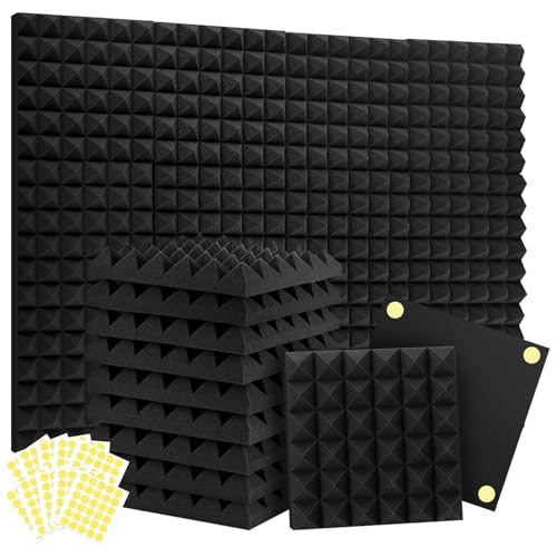
Focusound Acoustic Panels 24 Pack 2"x12"x12" with 120 PCS Double-Side Adhesive - Sound Proof Pyramid Foam for Walls, Home Studio Noise Absorption & Echo Control Kit

Dense foam damping axial modes — place at pressure antinodes displayed in room-mode visualizer's 3D pressure field.

$27.98 USDView ↗

$229.99Audio interface

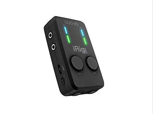
IK Multimedia iRig Pro Duo I/O USB audio interface, TRS balanced & headphones outputs, audio mixer to 24-bit, midi interface for music studio, recording, podcasting, streaming & social apps

Portable 2-channel USB-C audio interface used for mobile Biquadia field recording.

DSP · Audio

$229.99 USDView ↗

$71.89Book

Immersive Sound: The Art and Science of Binaural and Multi-Channel Audio (Audio Engineering Society Presents)

Derives HRTF, ITD = d/c sinθ, and head-tracking compensation — the exact panning law this playground interpolates as you drag yaw.

DSP · Audio

$71.89 USDView ↗

$43.15Book

Master Handbook of Acoustics, Seventh Edition

Bible of RT60, Sabine, and absorption coefficients — the exact formulas these acoustic calculators implement for reverb, room modes, and critical distance.

$43.15 USDView ↗

$139.98Microphone

miniDSP UMIK-1 USB Measurement Calibrated Microphone

Calibrated USB mic with individual cal file — measure your room's RT60 and modal peaks to validate the room-mode eigenfrequencies this calculator predicts.

DSP · Audio

$139.98 USDView ↗

$157.00Microphone

RØDE NT-USB+ Professional-Grade USB Condenser Microphone For Recording Studio Quality Audio Directly To A Computer Or Mobile Device, Black

USB condenser mic used for nymic testing.

DSP · Audio

$157.00 USDView ↗

$8.99Audio

SABRENT USB External Stereo Sound Adapter for Windows and Mac. Plug and Play No Drivers Needed. (AU-MMSA)

USB audio interface used in early Biquadia MEMS-mic prototyping.

DSP · Audio

$8.99 USDView ↗

$299.99Microphone

Sennheiser Pro Audio Sennheiser Pro Audio Wireless Microphone System, Black (MKE600)

Wireless mic system used for akous's ambient/binaural field recording.

DSP · Audio

$299.99 USDView ↗

$319.00Microphone

Shure MV7+ Podcast Dynamic Microphone with Stand – OBS Certified, Enhanced Audio, LED Panel, USB-C & XLR Outputs, Auto Level Mode, Digital Pop Filter – for Podcasting, Streaming, and Recording, Black

USB/XLR hybrid mic used building and testing nymic.

DSP · Audio

$319.00 USDView ↗

$237.00Microphone

Shure MV88+ Video Kit Digital Stereo Condenser Microphone for iPhone, Android, Mac & PC - Portable Recording Mic with DSP Controls, Headphone Monitoring & Tripod, Black

Portable stereo condenser mic kit used for Biquadia field/video capture.

DSP · Audio

$237.00 USDView ↗

$113.00Headphones

Sony MDR7506 Professional Large Diaphragm Headphone

Reference studio headphones used for akous's binaural audio testing.

DSP · Audio

$113.00 USDView ↗

$100.39Book

The Physics of Musical Instruments

Modal analysis of plates and strings with Bessel functions — root of Chladni plate eigenmodes and waveguide modal cutoff fc = c/2a this toolbox computes.

$100.39 USDView ↗

Prices shown were retrieved from the Amazon Product Advertising API on 19 July 2026 and are indicative only — the price and availability on Amazon at the time of purchase apply.

More gear across every app: the full Gear list →

Two gotchas worth knowing

The rigid-wall assumption breaks at the first drywall

This tool assumes perfectly rigid walls — the Neumann boundary condition. Drywall on studs is not rigid; it's a compliant panel that shifts eigenfrequencies down by 2–5% and adds damping (finite Q). A mode computed at 42.9 Hz may measure at 40.5 Hz in a real room. The ordering and nodal geometry remain correct, but don't trust the absolute frequency to better than ±5%. If you need measurement-grade accuracy, use a calibrated mic and swept sine — the map is for placement decisions, not absolute frequency confirmation.

The 2D map is a single z-slice illusion

The pressure map shows a horizontal slice at the listener's ear height. But room modes are fully 3D — a mode you see as "null at center" on the 2D map may actually peak at z=1.80 m (standing height) while vanishing at z=1.20 m (sitting height). Oblique modes especially have strong z-dependence. If you move your measurement mic vertically and the boom returns, you're seeing exactly this effect. The table's "Pressure at listener" column uses all three coordinates, so it's always correct — trust the number, not just the 2D visual.

Hardware Rigs & Field Notes

Hardware build / Mic arrays

Real-Time Acoustic Beamforming on an iPhone with miniDSP UMA-8

Live SRP-PHAT direction finding, superdirective MVDR beamforming on a 44 mm ring, and physical directivity limits.

Hardware build / Measurement

Headphone Measurement with a Binaural Head: HD 650 + UMC1820

HATS measurement rig, true-RMS multimeter calibration under load, and per-ear swept-sine transfer functions.

JavaScript — the mode solver

The core roomModes() and modePressure() functions. Exhaustive integer scan, temperature-dependent speed of sound, zero-allocation cosine evaluation.

Room modes — JavaScript

const speedOfSound = (tC) => 331.3 * Math.sqrt(1 + tC / 273.15);

const schroederFrequency = (V, T60) => {
  if (V <= 0 || T60 <= 0) return NaN;
  return 2000 * Math.sqrt(T60 / V);
};

const modePressure = (x, y, z, Lx, Ly, Lz, nx, ny, nz) => {
  return Math.cos(nx * Math.PI * x / Lx)
       * Math.cos(ny * Math.PI * y / Ly)
       * Math.cos(nz * Math.PI * z / Lz);
};

const roomModes = (Lx, Ly, Lz, c, fmax) => {
  const modes = [];
  const maxNx = Math.ceil(2 * Lx * fmax / c) + 1;
  const maxNy = Math.ceil(2 * Ly * fmax / c) + 1;
  const maxNz = Math.ceil(2 * Lz * fmax / c) + 1;

  for (let nx = 0; nx <= maxNx; nx++) {
    const fx = (nx * c) / (2 * Lx);
    if (fx > fmax) break;
    for (let ny = 0; ny <= maxNy; ny++) {
      const fy = (ny * c) / (2 * Ly);
      if (Math.hypot(fx, fy) > fmax) break;
      for (let nz = 0; nz <= maxNz; nz++) {
        if (nx === 0 && ny === 0 && nz === 0) continue;
        const f = (c / 2) * Math.sqrt(
          (nx / Lx) ** 2 + (ny / Ly) ** 2 + (nz / Lz) ** 2
        );
        if (f > fmax) break;
        const nonZero = (nx > 0 ? 1 : 0) + (ny > 0 ? 1 : 0) + (nz > 0 ? 1 : 0);
        const type = nonZero === 1 ? 'axial'
          : nonZero === 2 ? 'tangential' : 'oblique';
        modes.push({ nx, ny, nz, freq: f, type });
      }
    }
  }
  return modes.sort((a, b) => a.freq - b.freq);
};

Frequently asked questions

Why are axial modes the loudest and most problematic?

Axial modes bounce between only two parallel walls — they touch the least total surface area per cycle and therefore lose the least energy to wall absorption. Tangential (four walls) and oblique (all six surfaces) leak energy faster because every wall contact bleeds a small fraction. In a concrete room, the (1,0,0) axial at c/(2Lx) is almost always the worst offender — it's the one you hear booming when you clap.

How do I read the pressure at listener column?

It's the eigenfunction value p(x,y,z) at your listening position, ranging from -1 (antinode with inverted phase) to +1 (antinode). Values near 0 mean you're sitting in that mode's pressure null — you won't hear that frequency even if the source is exciting it. Values above 0.5 in magnitude mean that mode dominates your seat. Scan the table: modes with |p| > 0.5 are the ones you need to treat or move away from.

What should I do with the Schroeder frequency number?

Below fs, individual modes are sparse and audible — treat them with tuned traps, sub/listener placement, or narrow EQ cuts. Above fs, modes overlap densely and behave statistically — broadband absorption works. The tool estimates T₆₀ from Sabine with ᾱ=0.15 (typical furnished room). If your room is more absorbent, fs shifts down; if it's concrete, fs shifts up. Measure T₆₀ to get the real crossover.

Why do my measured room modes differ from the calculator's predictions?

Several reasons: real walls are not perfectly rigid (they're compliant, shifting frequencies down 2-5%), absorption isn't uniform across surfaces, furniture breaks the modal cosine shape, and non-rectangular geometry (alcoves, sloped ceilings) breaks the integer-index assumption entirely. This tool gives the rigid-wall ideal — it's typically within 5% for concrete rooms and serves as an excellent starting point for placement decisions even in imperfect rooms.

How do I use the 2D pressure map to place a subwoofer?

Select a problematic mode from the dropdown, then look for red or blue regions — those are pressure antinodes (walls and certain interior regions where cosines peak). Placing a sub in an antinode maximally excites that mode. If you want to kill the mode instead, place the sub at a white/light region (pressure node) where cos≈0 — the sub physically cannot couple to that mode. Move the listener dot similarly: put your head in a zero-pressure region for that frequency and you won't hear it.

Shareable still

The instrument, captured—not illustrated.

This 16:9 frame is rendered from the real browser instrument above. It is the page's canonical preview for image search, link unfurls, and posts that need to show what the tool actually does.

Download 1280 × 720 JPEG

Room Mode Calculator — live MakerPortal instrument screenshot — Canonical capture · real UI · no generated scientific artwork

← All Lab Field notes