Playground · research instrument
SignalSmith Chart Calculator
A microwave workbench in your browser: Smith Chart rotation, stub tuning (open/short electrical deg + position), L-network with series L/C shunt C/L, live S11/S21 sweep 0.1–6 GHz, matching journey trace, schematic view, and sonification where wideband hiss collapses to a pure 440 Hz when you hit 50 Ω (VSWR→1).
Independent research instrument — not claimed as MakerPortal shipped product code. Methods, equations, assumptions, and limitations are disclosed so you can inspect what the page does and does not establish.
Impedances
Source Zₛ = Rₛ + j Xₛ (ref)
Load Zʟ = Rʟ + j Xʟ
Matching Network
Bandwidth of noise ∝ |Γ|·2 kHz, Q=0.5+(1-|Γ|)·28. When |Γ|→0, tone 440 Hz pure, VSWR≈1. Bar shows match % = 100·(1-|Γ|).
Smith Chart 400×400 — normalized to Z₀
|Γ₀|=—Gold = ΓL, Cyan = after line, Orange = after stub, White = final. Spiral = sweep 0.1–6 GHz. Dashed = VSWR=2 circle. Click near center to snap load 50Ω.
Matching Network Schematic — live
S-Parameters vs Frequency — S11 red, S21 blue (lossless est)
f0 markerAnatomy of the bench
Signal path & controls
- Source Zₛ = Rₛ+jXₛ: reference for Smith normalization. Default 50+ j0. Changing Rₛ moves VSWR circles scaling. Xₛ is used for conjugate matching target Rₛ−jXₛ.
- Load Z_L: R_L 5–300Ω, X_L −200→+200Ω. Directly drives Γ_L=(Z_L−Z0)/(Z_L+Z0). Gold dot on Smith.
- Line to stub d: position from load in λ at f₀: βl_pos0=2π·d/λ. Frequency scaling βl(f)=βl0·f/f0 rotates Γ: Γ1=ΓL·exp(-j2βl). Cyan dot. Visual arc is constant |Γ|.
- Stub susceptance: shunt stub at distance d. Open B=Y0·tanθ_s, Short B=−Y0·cotθ_s where θ_s electrical length slider. At f, θ_s(f)=θ_s0·f/f0. Admittance Y2=Y1+jB. Moves along constant conductance circle (orange).
- L-network: two reactive elements. Auto solver picks shunt-first if Re(Z2)>Rs else series-first. For shunt-first, G/D=Rs gives B = −B_L ±√(G_L/Rs−G_L²). X = (B_L+B)/D − Xs. Sign of X,B decides L (positive) vs C (negative). Schematic shows coil vs capacitor. Final white dot near center when matched.
Line transformation
Clockwise rotation on Smith with line length. Sweep over f traces spiral.
Visualization & audio coupling
- Smith 400×400: resistance circles r=0,0.2,0.5,1,2,5 centered at r/(1+r) radius 1/(1+r). Reactance circles ±x with centers 1±j/x. VSWR=2 circle radius 1/3. Sweep trace blue thin line from 0.1–6 GHz computed with frequency-scaled βl. Journey polyline gold→cyan→orange→white with arrow.
- S-param sweep 900×280: log-ish linear f axis. S11_dB=20log10|Γ(f)| clipped −40→0 dB. S21_dB=10log10(1−|Γ|²) for lossless estimate. Current f0 marker white dot, green dashed −10 dB bandwidth crossing.
- Schematic: Canvas 520×400 draws source circle left, series element (zig inductor if X>0 else two plates for C with value), shunt to ground mid with component, transmission line as two parallel lines length ∝ d, stub perpendicular length ∝ θ_e with open circle or ground short, load resistor zigzag with label matched %. Label Q=√(Rp/Rs−1).
- Audio engine: white noise buffer loop → Biquad bandpass fc=440 Hz Q=0.5+(1−|Γ|)·28 → gain noise =0.05+|Γ|·0.18. Pure tone osc 440 Hz gain =(1−|Γ|)²·0.28, beat osc 440+|Γ|·38 Hz gain |Γ|·0.13 creates hum beating off-match. Two extra hum oscs 120 Hz & 185 Hz gains ∝|Γ| fade as matched. When VSWR≈1 ( |Γ| < 0.02 ) noise → narrow hum resolving to clean single 440 Hz.
Stub + L-match Q
Gear behind this build
RF stack · 5 picks
RF & Microwave instruments5
 $233.00Book
Microwave Engineering
Derives S-parameter conversion Z=Z0(I+S)(I-S)^-1, Smith Chart mapping Γ=(Z-Z0)/(Z+Z0), and stub matching l=λ/2π arctan(B/Y0) this bench solves continuously during drag.
 $85.49Diagnostic
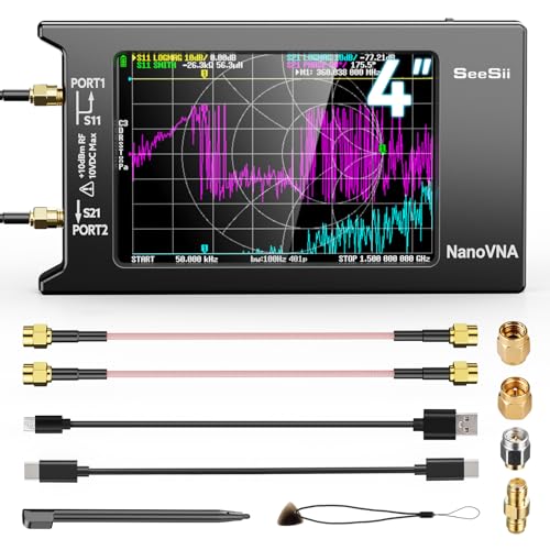
SEESII Upgraded NanoVNA-H4 Vector Network Analyzer, Latest V4.4 9KHz-1.5GHz HF VHF UHF 4" Touch Screen VNA Antenna Analyzer Measures S Parameters,Voltage Standing Wave Ratio, Phase,Delay, Smith Chart
Handheld VNA with touchscreen + SOL kit — S11/S21 lab companion for RF Bench and Antenna Sandbox.
 $38.32Book
RF Circuit Design
L-network matching Q = sqrt(Rp/Rs-1) and component X = ±Q*Rs formulas — this bench's auto-match button solves these analytically then animates Smith Chart journey through series L then shunt C.
 $13.90Kit
AURSINC SMA Calibration Kit and SMA Male to Male Jumper for NanoVNA H H4 F V2 V3 SAA Mini1300 PS100 Vector Network Analyzer Antenna Analyzer
SOL cal standards + SMA jumper for NanoVNA H/H4 — SI Lab and RF Bench SOLT demos.
 $206.99Diagnostic
AURSINC TinySA Ultra+ ZS406 Spectrum Analyzer with 50W N-Type RF Attenuator
Portable spectrum analyzer + attenuator kit — EMI and spur checks next to the RF Bench.
Prices shown were retrieved from the Amazon Product Advertising API on 8 October 2026 and are indicative only — the price and availability on Amazon at the time of purchase apply.
More gear across every app: the full Gear list →
Hardware Kit Builder
Build the physical hardware platform. Select your components below to generate a live, real-time bill of materials and build instructions.
Build this lab
RF bench starter
NanoVNA + SOL cal + Bowick — close the loop on RF Bench plots. Add TinySA or Pozar when you need spectrum / deeper theory.
- $85
- $14
- $38
- $207
- $233
Prices shown were retrieved from the Amazon Product Advertising API on 8 October 2026 and are indicative only — the price and availability on Amazon at the time of purchase apply.
Estimated total
$138
Prices from Amazon catalog cache · may change
Equations
Reflection
Line + Stub
L-Match Q & components
Core solver — TypeScript
// Complex helpers
type C = { re:number; im:number };
export const c = (re:number, im=0):C => ({re,im});
export const cAdd = (a:C,b:C):C => ({re:a.re+b.re, im:a.im+b.im});
export const cSub = (a:C,b:C):C => ({re:a.re-b.re, im:a.im-b.im});
export const cMul = (a:C,b:C):C => ({re:a.re*b.re-a.im*b.im, im:a.re*b.im+a.im*b.re});
export const cDiv = (a:C,b:C):C => {
  const d=b.re*b.re+b.im*b.im||1e-12;
  return {re:(a.re*b.re+a.im*b.im)/d, im:(a.im*b.re-a.re*b.im)/d};
};
export const cMag = (a:C) => Math.hypot(a.re,a.im);
export const cInv = (a:C):C => cDiv(c(1,0), a);

// Reflection
export function Gamma(Z:C, Z0:number):C {
  return cDiv(cSub(Z,c(Z0,0)), cAdd(Z,c(Z0,0)));
}

// Zin through lossless line: Z0*(ZL + j Z0 t)/(Z0 + j ZL t), t=tan(beta l)
export function Zin_line(ZL:C, Z0:number, tanBL:number):C {
  // numer = ZL + j Z0 t
  const numer: C = {re: ZL.re, im: ZL.im + Z0*tanBL};
  // denom = Z0 + j ZL t = (Z0 - XL*t) + j RL*t
  const denom: C = {re: Z0 - ZL.im*tanBL, im: ZL.re*tanBL};
  const ratio = cDiv(numer, denom);
  return {re: ratio.re*Z0, im: ratio.im*Z0};
}

// Stub susceptance: Y0=1/Z0
export function stubSus(Y0:number, betaL:number, type:'open'|'short'):number {
  const t = Math.tan(betaL);
  if(type==='open') return Y0 * t; // B
  // short: -Y0 cot = -Y0 / tan
  return Math.abs(t) < 1e-5 ? -Y0*1e3*Math.sign(t||1) : -Y0 / t;
}

// L-match Q (XL=0 case)
export function lMatchQ(Rp:number, Rs:number):number {
  return Math.sqrt(Math.max(0, Rp/Rs - 1));
}

// Shunt-first solution for target Rs (real), source Xs=0 simplified
export function designShuntFirst(ZL:C, Rs:number){
  const YL = cInv(ZL); // G+jB
  const GL = YL.re, BL = YL.im;
  const disc = GL/Rs - GL*GL;
  if(disc < 0) return null;
  const sq = Math.sqrt(disc);
  const B1 = -BL + sq, B2 = -BL - sq;
  const D1 = GL*GL + (BL+B1)*(BL+B1), D2 = GL*GL + (BL+B2)*(BL+B2);
  const X1 = (BL+B1)/D1, X2 = (BL+B2)/D2;
  return [{B:B1,X:X1},{B:B2,X:X2}];
}
Frequently asked questions
What exactly is plotted on the Smith Chart here?
Smith Chart maps normalized impedance z=Z/Z0 to reflection Γ=(z-1)/(z+1). We use Z0=50 Ω (or source Rs if you change it). Load ZL gives ΓL. Transmission line of electrical length θ=βl rotates Γ by e^{-j2θ}: Γ_in = ΓL·e^{-j2θ} moving clockwise on constant |Γ| circle. Adding a shunt stub adds susceptance jB moving along constant conductance circle. L-network then adds series jX and shunt jB to bring Γ to origin (50Ω). The trace shows sweep vs frequency and the matching journey with animated rotation as you tune stub.
How does stub susceptance work? Open vs short?
For lossless line, open stub Zin_open = -j Z0 cot βl_stub → Yin = j Y0 tan βl. So susceptance B_open = Y0·tan βl, can be capacitive (0<θ<90°) or inductive. Short stub Zin_short = j Z0 tan βl → Yin = -j Y0 cot βl, B_short = -Y0·cot βl. At θ=45°, open gives +Y0 (cap), short gives -Y0 (ind). At 90°, open → ∞ susceptance (short circuit), short → 0 (open). We clamp near singularities.
What formula does the auto L-match use?
Two topologies. Shunt-first (RL>RS): given G_L+jB_L=1/Z_mid, we need G_L/D=1/RS where D=G_L²+(B_L+B)² → B = -B_L ± sqrt(G_L/RS - G_L²). Then series X = (B_L+B)/D - XS to cancel source reactance. Series-first (RL<RS): RL²+(XL+X)² = RL·(RS²+XS²)/RS → X = -XL ± sqrt(...), then B = B_target - B' where B_target = XS/(RS²+XS²). The simpler textbook Q for XL=0: Q=√(Rp/Rs -1), with Rp larger R. Then series X=Q·Rs, shunt susceptance Q/Rp. Two sign solutions map to low-pass (L in series, C shunt) vs high-pass.
How is S11 / S21 computed across frequency?
For each f in 0.1–6 GHz sweep, βl = θ0·f/f0 where θ0 is electrical length at f0 (center). Stub length θ_stub(f)=θ_stub0·f/f0. Transform ZL through line length pos: Z1=Z0·(ZL+jZ0 tan βl_pos)/(Z0+jZL tan βl_pos). Add stub: Y2=Y1+jB_stub(f), Z2=1/Y2. Apply L-match frequency scaling: if series L: X(f)=X0·f/f0, if C: X0·f0/f. Shunt B(f): if C: B0·f/f0, if L: B0·f0/f. Then get Z_in(f). Γ(f)=(Z_in-Z0)/(Z_in+Z0). S11=20log10|Γ|. For lossless network, S21=10log10(1-|Γ|²) = insertion loss; we plot that as transmission. VSWR=(1+|Γ|)/(1-|Γ|).
Why does the audio go from noisy hum to pure 440 Hz?
Web Audio: white-noise buffer (2s loop) → Biquad bandpass centered 440 Hz with Q = 0.5 + (1-|Γ|)·28. Bandwidth BW = fc/Q. When |Γ|≈1 wideband (Q low) → harsh multi-frequency hiss representing mismatch. When |Γ|→0, Q→28 → narrow hum around 440 Hz. Simultaneously two tone oscillators: pure 440 Hz gain = (1-|Γ|)²·0.28, beat oscillator 440+|Γ|·38 Hz gain = |Γ|·0.13 creates beating when mismatched. At |Γ|<0.02 (VSWR≈1.04) only 440 remains, indicating 50 Ω lock. Extra 120 Hz and 185 Hz hum oscillators faded by |Γ| give power-line-like hum off-match.
Shareable still
The instrument, captured—not illustrated.
This 16:9 frame is rendered from the real browser instrument above. It is the page's canonical preview for image search, link unfurls, and posts that need to show what the tool actually does.
Download 1280 × 720 JPEG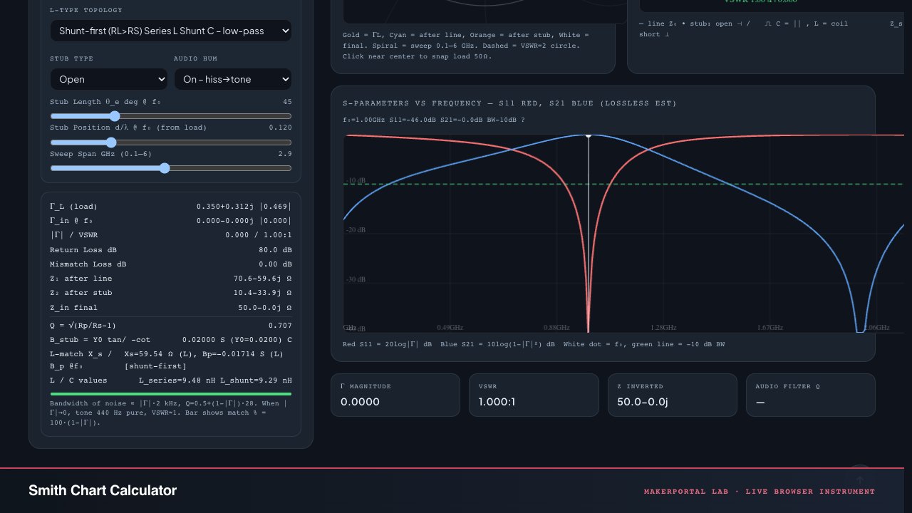
Continue the experiment