Playground · research instrument

ABCD Matrix Calculator

Build an optical system out of lenses, mirrors, and gaps, and watch a fan of paraxial rays trace straight through it. Every element is a 2×2 ABCD matrix; the whole cascade collapses to one matrix whose effective focal length and imaging conjugates are read out live. A second mode tests two-mirror laser cavities against the classic g1·g2 stability criterion.

Independent research instrument — not claimed as MakerPortal shipped product code. Methods, equations, assumptions, and limitations are disclosed so you can inspect what the page does and does not establish.

Elements

light travels left → right

Input rays

Beam half-height (mm)10

Presets

Hardware hook:Get the Optical Bench Rail with Lens and Mirror Set ↗

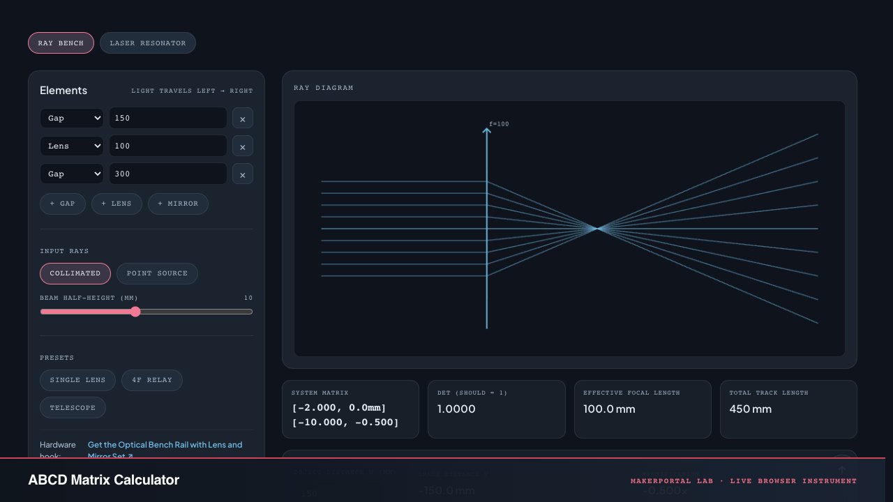
Ray diagram

System matrix

[-2.000, 0.0mm]
[-10.000, -0.500]

det (should = 1)

1.0000

Effective focal length

100.0 mm

Total track length

450 mm

Object distance u (mm)

Image distance v

-150.0 mm

Magnification

-0.500×

Anatomy of the instrument

Every pixel above answers to the math below. Here is what each piece of the two-panel instrument is actually doing, and why it is built that way.

The ray-bench canvas

01
Optical axis and grid. The horizontal centerline is the optical axis ( $y=0$ ). The canvas auto-scales its vertical extent so the outermost ray never clips, and the axis stays centered regardless of element count or fan width.
02
Lens markers. Converging lenses ( $f > 0$ ) show convex arrowheads pointing outward; diverging ( $f < 0$ ) show concave arrowheads pointing inward. Colour is the anchor blue. A label "f=" marks the focal length in mm.
03
Mirror lines. Curved mirrors are drawn at their unfolded position (the reflection is folded into the forward-propagating convention). Convex/concave is shown via the R= label; colour is the brand pink. A flat mirror ( $R \to \infty$ ) collapses to the identity matrix and draws no optical power, so a cavity with $R=\pm400$ is functionally flat here.
04
Ray traces. Nine rays per mode. Collimated mode fans a range of input heights at $\theta=0$ ; point-source mode fans a range of angles from $y=0$ . Each ray is stepped element-by-element through traceRay() — no approximation besides the paraxial limit built into the matrices themselves.
05
Element cascade (matrix multiplication order). The system matrix is built as $M_{\text{sys}} = M_n \cdots M_2 M_1$ where $M_1$ is the first element light hits (rightmost in the product). Each added element left-multiplies the accumulator. The order is not commutative — reversing it gives wrong physics, as the gotchas below explain.

Controls, readouts, and cavity mode

01
Element types. Gap is freeSpace(d) with matrix $\begin{bmatrix}1 & d \\ 0 & 1\end{bmatrix}$ . Lens is thinLens(f) with matrix $\begin{bmatrix}1 & 0 \\ -1/f & 1\end{bmatrix}$ . Mirror is curvedMirror(R) with $C = -2/R$ , effectively a lens of $f = R/2$ . All values in mm on the UI, converted to meters for the optics functions.
02
Presets. Single lens ( $f=100$ mm, $u=150$ mm), 4f relay (two $f=100$ mm lenses separated by $2f$ — unity magnification, afocal), and Keplerian telescope ( $f_1=200,\, f_2=50$ mm separated by $f_1 + f_2$ ). Click any preset to load its elements and redraw.
03
Readouts. System matrix $[A, B; C, D]$ with $B$ in mm, determinant $AD - BC$ (should read 1), effective focal length $EFL = -1/C$ (shows "afocal" if $C=0$ ), total track length. The imaging panel below solves $B=0$ for image distance $v$ given object distance $u$ and the system matrix.
04
Cavity mode. The second tab computes the round-trip matrix through two mirrors plus free space, extracts $g_1, g_2$ and their product, checks stability, and plots the cavity on the $(g_1, g_2)$ plane with the hyperbolic stable region shaded. Edge cavities ( $g_1 g_2 \approx 0$ or $\approx 1$ ) show "edge" in place of beam sizes — the Gaussian mode diverges at the boundary.
05
Render loop. There is no idle requestAnimationFrame spin. The canvases re-render on any element change, slider move, preset load, tab switch, or theme mutation. The pixel-shaded stability region on the cavity canvas is pre-computed into an ImageData buffer each render — no per-pixel math during idle.

The ABCD matrix cascade

M_{\text{sys}} = M_n \cdots M_2 M_1 = \begin{bmatrix} A & B \\ C & D \end{bmatrix}

The image-formation condition $B = 0$ yields $v = -A / C$ . Magnification is the $A$ element of the full object-to-image matrix: $M = \operatorname{FreeSpace}(v) \cdot M_{\text{sys}} \cdot \operatorname{FreeSpace}(u)$ . If $C = 0$ the system is afocal — no real image forms at finite distance.

Gear behind this build

Optics bench stack · 7 picks

Optics hardware7

$89.70Kit

DKULMN Physical Optics Experimental Equipment, Concave-Convex Lens and Large Optical Bench,Optical Bench Set,Complete Teaching Equipment

1-meter rail with carriers for lenses/mirrors — recreate the resonator stability test g1·g2 and image formation this simulator ray-traces via ABCD multiplication.

$89.70 USDView ↗

$213.49Apparatus

Eisco - Complete Optical Bench and Attachment Set with 40 Pieces and 20 Lab Activities for Optics Experiments

Actually a wind-tunnel-friendly flow-viz partner — pair with smoke tube to see boundary-layer separation and wake shedding your D2Q9 simulation traces numerically.

$213.49 USDView ↗

$193.68Book

Fundamentals of Photonics

Derives Gaussian beam resonator stability and ABCD law for laser cavities — test the g1·g2 ≤1 condition this bench evaluates for two-mirror resonators.

$193.68 USDView ↗

$41.99Kit

GeRRiT Physical Optical Equipment Set Science Classroom Optics Kit Concave Convex Lens Optical Bench Attachment Set Complete Optical Teaching Equipment Physical Imaging Equipment for Laboratory

Handheld concave/convex lenses and ray box — build the same ABCD cascade (lens-gap-mirror) physically and verify the numerical ray fan traced here.

$41.99 USDView ↗

$237.23Book

Optics

Chapter 6 derives the 2×2 ABCD matrix for lenses/mirrors — the exact paraxial ray transfer this bench composes to build system matrix and effective focal length.

$237.23 USDView ↗

$53.90Book

Optics Global Edition

Covers g1·g2 resonator stability criterion |g1 g2| ≤ 1 — toggle the two-mirror cavity in this bench and watch stable/unstable regions match Hecht's diagram.

$53.90 USDView ↗

$Principles of Optics: Electromagnetic Theory of Propagation, Interference and Diffraction of Light$ $59.69Book

Principles of Optics: Electromagnetic Theory of Propagation, Interference and Diffraction of Light

Rigorous electromagnetic theory of ABCD and Fresnel diffraction — compare paraxial ray fan this bench traces to Born's exact wavefront aberrations.

$59.69 USDView ↗

Prices shown were retrieved from the Amazon Product Advertising API on 19 July 2026 and are indicative only — the price and availability on Amazon at the time of purchase apply.

More gear across every app: the full Gear list →

Method & limitations

Paraxial optics looks like a trick: take a messy pile of glass and empty space and crush it into one $2 \times 2$ matrix. That matrix tells you where any ray goes. No wave integrals, no Snell's law at each surface. If a ray stays close to the axis and shallow, two numbers are enough — height and slope — and every element is just a linear nudge on that pair.

What the math is

A ray is $\begin{bmatrix} y \\ \theta \end{bmatrix}$ . $y$ is transverse height in meters, $\theta$ is slope in radians, with $\sin\theta \approx \theta$ . That is the whole state. Propagation does not need calculus — it is matrix multiplication.

Free space of length $d$ : $\begin{bmatrix} 1 & d \\ 0 & 1 \end{bmatrix}$ . Intuition: $y' = y + d\theta$ , height grows proportional to slope times distance, slope unchanged. If you coast, you drift up if you were pointing up.

Thin lens of focal length $f$ : $\begin{bmatrix} 1 & 0 \\ -1/f & 1 \end{bmatrix}$ . Height unchanged entering the glass, slope gets a kick $\Delta\theta = -y/f$ . Positive $f$ bends inward, negative bends outward. It is literally a proportional controller on height.

Curved mirror radius $R$ : unfold the reflection and it looks identical to a lens. $C = -2/R$ , so $f = R/2$ . Concave toward incoming light is positive $R$ and focusing. Flat mirror is identity — $R \to \infty$ makes $C \to 0$ .

Cascade: $M_{sys} = M_n \cdots M_2 M_1$ . Order matters. First element is rightmost. Multiply them all, you get one matrix with elements $A, B, C, D$. If input and output media match, $\det M_{sys} = AD - BC = 1$ . That is not numerology — it is conservation of etendue in first order, and your first debug check.

Effective focal length falls out immediately: $EFL = -1/C$ . Why? Send in a collimated ray with $\theta=0$ , height $y$ . Output slope is $C y$. Focal point is where that ray crosses the axis, at $y / |\theta'| = -1/C$ . If $C=0$ , system is afocal — telescope, 4f relay. Collimated in, collimated out.

What it ignores

This is strictly paraxial, first-order optics: small angles only, no aberrations (spherical, coma, astigmatism, chromatic), no diffraction at apertures, and thin elements unless you build a thick lens from two refracting interfaces. Ray heights in the diagram are exaggerated for visibility — the math still assumes $\theta \ll 1$ rad.

No aberration theory. Real lenses smear focus; ABCD imagines perfect conics focused to a point.
No stop, vignetting, or diffraction. A 10 mm "beam" here would clip in hardware; here it traces forever.
No dispersion. $n(\lambda)$ is constant in this model, so chromatic focal shift is absent.
No polarization or coatings. Fresnel loss and phase on reflection are not tracked.

It is exact in the paraxial limit and ideal for layout, first-order imaging conjugates, and cavity architecture, but it is not a replacement for sequential ray-tracing or wave-optics propagation when you care about spot quality.

Resonator stability

When does a photon stay in the box?

For two mirrors separated by $L$ , define $g_i = 1 - L/R_i$ . This single number captures geometry: flat mirror has $g=1$ , confocal $R=L$ gives $g=0$ , concentric $R=L/2$ gives $g=-1$ .

Trace a ray one round trip: $M_{rt} = M(R_1) \cdot P(L) \cdot M(R_2) \cdot P(L)$ . Stability asks whether repeated application blows up or stays bounded. Eigenvalue analysis of a $2\times2$ symplectic matrix gives the clean criterion $0 \le g_1 g_2 \le 1$ . Inside: bounded, Gaussian eigenmode exists. Outside: walk-off. Edge cases — plane-parallel $g_1 g_2=1$ and confocal $g_1 g_2=0$ — are marginally stable in theory, alignment-sensitive in practice.

Equivalent form: $|(A+D)/2| \le 1$ , where $M_{rt} = \begin{bmatrix} A & B \\ C & D \end{bmatrix}$ . We evaluate both so you can see they agree. The canvas plots $(g_1,g_2)$ with the stable hyperbolic region shaded.

Gaussian beams — beyond rays

A complex number holds curvature and width

Geometrical rays say nothing about focus size. Gaussian optics fixes it with $q$ . Definition: $1/q = 1/R - i \lambda / (\pi w^2)$ , where $R$ is phase-front curvature, $w$ is $1/e^2$ radius. Imaginary part stores width, real part stores curvature.

Propagation law is identical in form to ray optics: $q' = (A q + B)/(C q + D)$ . That is not a coincidence — it is Collins diffraction integral evaluated for a Gaussian. At a waist $R=\infty$ , so $q = i z_R$ with Rayleigh range $z_R = \pi w_0^2 / \lambda$ .

In a stable resonator, demand $q$ reproduce itself after one round trip up to same $q$ . Solve $q = (A q + B)/(C q + D)$ with $M_{rt}$ . The resulting $w_0, w_1, w_2$ are what we display. When $g_1 g_2$ approaches 0 or 1, $w$ diverges — that is the physics telling you edge resonators have huge spots and tight tolerances.

Start with a free-space beam? The Gaussian beam calculator turns wavelength and waist into $z_R$ , divergence, spot size, curvature, and a scaled envelope before you add lenses here.

Solver lives in src/lib/optics.ts — pure functions, no DOM. Tested against thin-lens conjugate $1/u + 1/v = 1/f$ , combined focal lengths, confocal/planar edges $g_1 g_2$ , and Gaussian expansion $w(z_R)=\sqrt{2} w_0$ .

Two gotchas worth knowing

Paraxial rays only

The ABCD method replaces $\sin\theta \approx \theta$ and $\tan\theta \approx \theta$ , which holds to better than 1% for angles under about 8° (0.14 rad). Feed a 30° ray into these matrices and the output is not just wrong — it violates Snell's law entirely, since the matrix assumes linearity that only exists for small angles. The canvas exaggerates ray heights to fill the viewport; the math underneath still assumes shallow slopes. If your real system has steep bends, switch to sequential ray-tracing or a non-sequential Monte Carlo engine.

Matrix order is NOT commutative

$M_1 M_2 \neq M_2 M_1$ . The system matrix is built by left-multiplying each successive element: $M_{\text{sys}} = M_n \cdots M_2 M_1$ , where $M_1$ is the first element light hits. If you stack the element-dialog entries top-to-bottom but multiply them bottom-to-top, you have secretly reversed your optical train. The real consequence: a lens then a gap yields a different system matrix than a gap then a lens — and the focal point moves. The add-element buttons and preset loaders here always build in the correct left-to-right order, but if you reorder rows manually and don't understand the right-to-left multiplication convention, the readouts will silently disagree with your drawing.

TypeScript, the core engine

Three pure functions from src/lib/optics.ts do the heavy lifting. They have no DOM, no framework, no side effects — drop them into any TypeScript project.

systemMatrix · traceRay · effectiveFocalLength

export function systemMatrix(elements: Matrix2[]): Matrix2 {
  let m = { ...identity };
  for (const el of elements) m = multiply(el, m);
  return m;
}

export function traceRay(m: Matrix2, ray: Ray): Ray {
  return {
    y: m.A * ray.y + m.B * ray.theta,
    theta: m.C * ray.y + m.D * ray.theta,
  };
}

export function effectiveFocalLength(m: Matrix2): number {
  if (m.C === 0) return Infinity;
  return -1 / m.C;
}

Frequently asked questions

What is an ABCD ray-transfer matrix?

In paraxial (small-angle) optics a ray is described by its height y and slope θ. Every optical element — a length of free space, a thin lens, a curved mirror — acts on that pair through a 2×2 matrix [[A, B], [C, D]]. Cascading elements just multiplies their matrices, so an entire optical system collapses to a single 2×2 matrix. It is the standard first-order design tool for imaging systems and laser cavities.

What does the g₁·g₂ stability criterion mean?

For a two-mirror laser cavity define g₁ = 1 − L/R₁ and g₂ = 1 − L/R₂. The cavity is stable — rays stay bounded round-trip after round-trip — when 0 ≤ g₁·g₂ ≤ 1. Outside that region rays walk off the mirrors. Edge cases like plane-parallel (g₁·g₂ ≈ 1) and confocal (g₁·g₂ = 0) are sensitive to alignment in practice. The equivalent check on the round-trip matrix is |(A+D)/2| ≤ 1 and both are evaluated live in the resonator tab.

Why does the paraxial approximation work?

The paraxial approximation replaces sinθ with θ and tanθ with θ, which is accurate to better than 1% for angles under about 8° (0.14 rad). Since most imaging systems and laser cavities operate with shallow ray angles, this linearization captures real-world behavior remarkably well. It is what lets you replace Snell's law at each surface with a simple matrix multiplication.

How do real lenses differ from these ideal ABCD matrices?

The thin lens matrix assumes zero thickness and perfect focusing — no spherical aberration, no coma, no chromatic focal shift. A real lens has thickness, curved surfaces with higher-order figure errors, wavelength-dependent refractive index, and diffraction at its aperture. ABCD matrices give you the first-order layout (where things focus, magnification); a full ray-tracing or wave-optics package adds the aberrations on top.

Why should the determinant of the system matrix be 1?

For a system that begins and ends in the same medium (e.g. air → air), the determinant equals the ratio of input to output refractive index — unity. It is a useful numerical sanity check: if your cascade does not come out to det = AD − BC ≈ 1, an element value or ordering is wrong. Floating-point arithmetic may show 0.9999 or 1.0001 but a 0.5 or 2.0 means you lost a factor somewhere.

Shareable still

The instrument, captured—not illustrated.

This 16:9 frame is rendered from the real browser instrument above. It is the page's canonical preview for image search, link unfurls, and posts that need to show what the tool actually does.

Download 1280 × 720 JPEG

Ray-Matrix Optics Bench — live MakerPortal instrument screenshot — Canonical capture · real UI · no generated scientific artwork

Continue the experiment

All lab instruments →

Research

ABCD Matrix Calculator

Elements

Two-mirror cavity

Anatomy of the instrument

The ray-bench canvas

Controls, readouts, and cavity mode

Gear behind this build

Optics hardware7

DKULMN Physical Optics Experimental Equipment, Concave-Convex Lens and Large Optical Bench,Optical Bench Set,Complete Teaching Equipment

Eisco - Complete Optical Bench and Attachment Set with 40 Pieces and 20 Lab Activities for Optics Experiments

Fundamentals of Photonics

GeRRiT Physical Optical Equipment Set Science Classroom Optics Kit Concave Convex Lens Optical Bench Attachment Set Complete Optical Teaching Equipment Physical Imaging Equipment for Laboratory

Optics

Optics Global Edition

Principles of Optics: Electromagnetic Theory of Propagation, Interference and Diffraction of Light

Method & limitations

Two gotchas worth knowing

TypeScript, the core engine

Frequently asked questions

The instrument, captured—not illustrated.

Live Earth

Double Pendulum + Phase Space

Chladni Cymatics

ABCD Matrix Calculator

Optics bench

Elements

Two-mirror cavity

Anatomy of the instrument

The ray-bench canvas

Controls, readouts, and cavity mode

Gear behind this build

Optics hardware7

DKULMN Physical Optics Experimental Equipment, Concave-Convex Lens and Large Optical Bench,Optical Bench Set,Complete Teaching Equipment

Eisco - Complete Optical Bench and Attachment Set with 40 Pieces and 20 Lab Activities for Optics Experiments

Fundamentals of Photonics

GeRRiT Physical Optical Equipment Set Science Classroom Optics Kit Concave Convex Lens Optical Bench Attachment Set Complete Optical Teaching Equipment Physical Imaging Equipment for Laboratory

Optics

Optics Global Edition

Principles of Optics: Electromagnetic Theory of Propagation, Interference and Diffraction of Light

Method & limitations

Two gotchas worth knowing

TypeScript, the core engine

Frequently asked questions

The instrument, captured—not illustrated.

Related instruments

Live Earth

Double Pendulum + Phase Space

Chladni Cymatics