Playground · research instrument
On-device AISLAM Odometry Arena
EKF visual-inertial odometry in the browser: unicycle robot, IMU drift, range-bearing features, covariance ellipsoids, sparse 3-D point cloud, and bag-of-words loop closure that snaps the map with a spatial audio ping and viewport flash. Tune noise, watch ATE grow, close the loop.
Independent research instrument — not claimed as MakerPortal shipped product code. Methods, equations, assumptions, and limitations are disclosed so you can inspect what the page does and does not establish.
Odometry & Sensing
Motion model — IMU / wheel noise
Platform
Robot drives a noisy unicycle circle. EKF predicts with noisy v,w then updates with range-bearing landmarks. Uncertainty ellipsoids grow without loop closure — enable it and return to start to hear snap and see map correction.
Top-down arena — trajectory, landmarks, ellipsoids, loop edge
Sparse 3-D point cloud — pinhole projection from robot frame
Size ∝ 1/depth, color by visual word. Height jitter = stereo reconstruction noise.
Live histogram BoW
Visual words = 32 bins quantized by position hash. Loop when cosine similarity spikes as you revisit.
Anatomy of the arena
EKF SLAM pipeline
- State: μ ∈ R^(3+2N) = [x,y,θ, m1x,m1y…]. P covariance (3+2N)² initialized P_rr=0.01·I, P_mm=800·I for unknown landmarks.
- True world: N visual features uniformly in [-11,11]² with random height 0.3-2.4 m for cloud projection, descriptor = hash of cell + random BoW word in 0..31.
- Motion: unicycle v, ω. True integrates v, ω. Filter integrates v̂=v+𝒩(0,σ_m²), ω̂=ω+𝒩(0,(σ_m/2)²). Jacobian G = ∂f/∂[x,y,θ] = [[1,0,-v dt sinθ],[0,1,v dt cosθ],[0,0,1]]. P_rm = G P_rm.
- Observation: range r=√(dx²+dy²), bearing φ=atan2(dy,dx)−θ. ẑ = z_true+𝒩(0, diag(σ_o², (σ_o·0.6)²)). Only landmarks within range and |φ| < 95° generate measurement.
- Init: first sight sets μ_landmark = [x+ r cos(θ+φ), y+ r sin(θ+φ)], covariance clamped to 1.2, seen=true. Subsequent sights run sparse EKF update.
- Visualization: top-down shows true gray dots, estimated orange; ellipsoids 95% from marginal covariance. Robot triangle with σ ellipse. Odom-only (dead reckoning) dashed line diverges.
Motion Jacobian
Cross-covariance propagates by P_rm ← G P_rm keeping landmark correlations.
Loop closure, point cloud, audio
- Keyframes every ~1.1 m or 18° rotation: store pose, BoW 32-histogram, landmark IDs seen. History up to 90 frames.
- BoW similarity: cosine sim = (h1·h2)/(‖h1‖‖h2‖). Candidate if sim>0.72, metric distance of estimated trajectory loop <1.8 m, travelled >12 m, and not same recent frame.
- Correction: pose graph snap Δp=μ_kframe−μ_curr, applied 0.85 gain to μ_robot and shared landmarks shifted by Δp·0.7 averages (emulating BA). P_rr ×0.28 and P cross scaled 0.7 mimics information matrix boost.
- Feedback: flash overlay α flashTimer, canvas CSS translate jitter proportional to drift energy, loop edge green line, ATE drop in readout.
- Cloud projection: p_cam = R(-θ)([mₓ−x, mᵧ−y, h_z]ᵀ). u = cₓ + fₓ·pₓ/p_z, v = cᵧ − f_y·h_z/p_z, size ∝ 1/(p_z+0.2). Height noise simulated, size encodes depth uncertainty.
- Spatial audio: HRTF PannerNode. Pos = loop vector rotated into listener frame. Snap = 880 Hz sine ×exp(-18t) + 2.6 kHz pluck + 2-6 kHz noise burst 80 ms. Gain = 0.22 + 0.18·drift_before.
Observation Jacobian (one landmark)
q=dx²+dy², r=√q. Sparse so S is 2×2 only.
The math and physics, in full
EKF Predict
F_t = diag(G_t, I_2N). R_t only affects robot 3x3 block: sigma_v², sigma_w².
Range-bearing
EKF Update
H sparse 2×(3+2N). S⁻¹ analytic 2×2. Innovation angle wrapped to (−π,π].
95% ellipse
Loop & BA
Loop adds pose-pose constraint factor; BA optimizes over window. Filtering alone drifts O(√ distance).
Gear behind this build
SLAM stack · 11 picks
Hardware picks11
 $34.95Sensor
Adafruit 9-DOF Absolute Orientation IMU Fusion Breakout - BNO055
Bosch BNO055 fusion IMU breakout — quaternion/Euler output for flight, SLAM, and head-tracking labs. Closest verified Amazon listing to BNO085 workflows.
 Sensor
Intel RealSense Depth Camera D455
Stereo depth with IMU BMI055 fused via visual-inertial odometry — feed recorded bag into SLAM arena and validate simulated EKF reprojection error vs RealSense hardware baseline noise model.
 $399.00SBC
NVIDIA Jetson Orin Nano Super Developer Kit
67 TOPS edge AI dev kit — benchmark int4 quantized models sized here and validate that CoreML quantized size math predicts actual flash/RAM usage on device.
 $73.81Book
Multiple View Geometry in Computer Vision
Canonical multi-view geometry text underpinning visual odometry / SLAM pipelines.
 $259.95Sensor
SparkFun GPS-RTK-SMA Breakout - ZED-F9P (Qwiic)
SparkFun Original ZED-F9P RTK GNSS — centimeter-class pose for SLAM / odometry outdoor labs. 10% Originals commission.
 $20.95Sensor
SparkFun 9DoF IMU Breakout - ICM-20948 (Qwiic)
SparkFun Original Qwiic ICM-20948 — 9-DoF for PID Flight Arena and SLAM IMU fusion. 10% Originals commission.
 $249SBC
NVIDIA Jetson Orin Nano Super Developer Kit
Jetson Orin Nano Super via SparkFun — edge PINN / SLAM compute. Third-party NVIDIA kit (tracked referral).
 $259.95SBC
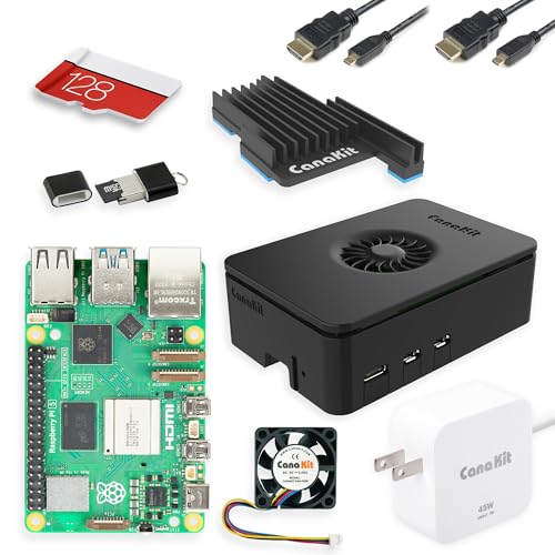
CanaKit Raspberry Pi 5 Starter Kit PRO - Turbine Black (128GB Edition) (8GB RAM)
Flagship Pi 5 8GB board — Amazon verified ASIN B0CK2FCG1K (via DuckDuckGo Amazon search). SparkFun third-party gave no commission; now Amazon affiliate.
 SBC
SBCSeeed Studio Raspberry Pi 5 Starter Kit - 16GB RAM, 64GBGB Micro SD Card Pre-Loaded 64-bit OS, Type-C Power Supply, Active Cooling Case for Edge AI, Docker & Pro Workstation
Pi 5 16GB starter kit — Amazon verified ASIN B0F944X9S4 (Seeed Studio 16GB + 64GB SD, Type-C PSU, case). 14.5 GiB ceiling for Q4_K_M up to ~12B params. SparkFun third-party gave no commission; now Amazon.
 $119.95Kit
Experiential Robotics Platform (XRP) Kit
SparkFun Original XRP robot kit — mechanical + control lab hardware when you outgrow FEA fixtures. 10% Originals. (No 3D printers in SparkFun catalog as of 2026-07.)
 $99.48Book
Probabilistic Robotics (Intelligent Robotics and Autonomous Agents series)
Bible for EKF-SLAM: Chapter 10 derives prediction x'=f(x,u)+w and update with Jacobian H and innovation y, covariance S = HPH^T+R, and loop-closure data association gating used live here.
Prices shown were retrieved from the Amazon Product Advertising API on 8 October 2026 and are indicative only — the price and availability on Amazon at the time of purchase apply.
Prices shown were each checked against the Amazon product listing between 8 August 2026 and 17 September 2026 and are indicative only — the price and availability on Amazon at the time of purchase apply.
More gear across every app: the full Gear list →
Hardware Kit Builder
Build the physical hardware platform. Select your components below to generate a live, real-time bill of materials and build instructions.
Build this lab
SLAM / odometry edge stack
Jetson + SparkFun ZED-F9P RTK + ICM-20948 — outdoor pose and onboard mapping. ZED-F9P and ICM are SparkFun Originals (10%).
- $249
- $260
- $21
- —
Prices shown were retrieved from the Amazon Product Advertising API on 8 October 2026 and are indicative only — the price and availability on Amazon at the time of purchase apply.
Estimated total
$530
Prices from Amazon catalog cache · may change
Core solver — TypeScript
// EKF SLAM minimal core: unicycle predict + sparse range-bearing update
type State = { mu: number[]; P: number[][]; seen: boolean[]; };

function predict(mu: number[], P: number[][], v: number, w: number, dt: number, q: number[]) {
  const th = mu[2];
  const G = [[1,0,-v*dt*Math.sin(th)],[0,1,v*dt*Math.cos(th)],[0,0,1]];
  // robot
  mu[0] += v*dt*Math.cos(th);
  mu[1] += v*dt*Math.sin(th);
  mu[2] += w*dt;
  // P_rr = G P_rr G^T + Q
  const Prr = [[P[0][0],P[0][1],P[0][2]],[P[1][0],P[1][1],P[1][2]],[P[2][0],P[2][1],P[2][2]]];
  const GP = matMul(G, Prr);
  const GPGT = matMul(GP, transpose(G));
  addDiag(GPGT, q); // Q = diag(motionNoise)
  // copy back + cross terms P_rm = G P_rm
}

function updateLandmark(mu: number[], P: number[][], zid: number, z: [number,number], R: number[][]){
  const rx=mu[0], ry=mu[1], rt=mu[2];
  const lix = 3+zid*2;
  const dx = mu[lix]-rx, dy = mu[lix+1]-ry;
  const q = dx*dx+dy*dy, r = Math.sqrt(q);
  const h = [r, Math.atan2(dy,dx)-rt];
  const Hr = [[-dx/r, -dy/r, 0],[ dy/q, -dx/q, -1]];
  const Hl = [[ dx/r,  dy/r],[-dy/q,  dx/q]];
  // sparse Jacobian 2x(3+2N) -> use only 5 columns
  // S = H P H^T + R (2x2), K = P H^T S^{-1}
  const innov = [z[0]-h[0], wrapAngle(z[1]-h[1])];
  // ... K, mu+=K*innov, P=(I-KH)P
  // loop closure: compare BoW histograms
}

function wrapAngle(a:number){ return Math.atan2(Math.sin(a), Math.cos(a)); }
Abridged: the Kalman gain, the covariance update and the loop-closure test are elided where the comments say so.
Export · Soft gate
Export EKF trajectory + landmarks
Robot poses (x,y,θ), covariance diag, loop-closure events as CSV — free watermarked, clean after email. Great for validating against RealSense D455 bag + ZED-F9P RTK ground truth.
File · slam-trajectory.csv
slam-trajectory.csvtext/csv+ watermark line on free pathFree download adds a small footer:
# Export from makerportal.ai — free watermarked build. Unlock c…Clean export removes footer. Both are generated fresh from your current sim tuning.
Privacy: email stays in your browser localStorage (mp_export_email_slam-odometry-arena) + unlock flag (mp_export_unlock_slam-odometry-arena). If Buttondown username is configured, we also POST to Buttondown (privacy-first mode, no tracking pixels per D-014). See privacy → affiliates & email.
Unlock clean export
Soft gate — no hard paywall, no Clerk. Email stays local unless you explicitly check the newsletter box. Unsubscribe anytime. RSS at /rss.xml.
✓ Lab Pro — clean export on every lab
Your licence unlocks this and every other gated simulator, so there is nothing to enter here. Manage or sign out on the shop page.
✓ Unlocked — clean exports enabled
Stored in mp_export_unlock_slam-odometry-arena. Clean file omits watermark. Re-lock via browser devtools → localStorage.
Frequently asked questions
What state does EKF-SLAM maintain?
μ = [x, y, θ, m1x, m1y, m2x, m2y, …]ᵀ dimension 3+2N. Covariance P is (3+2N)². Robot prediction uses differential-drive unicycle model, landmarks are static. Each range-bearing observation updates only 5 columns via sparse Jacobians, so S is 2×2 and K = P Hᵀ S⁻¹ can be formed from 5 columns of P.
How are uncertainty ellipses drawn?
For landmark j, marginal Σ = P[lm:lm+2, lm:lm+2] 2×2. Eigen-decomposition λ₁,₂ = (a+c)/2 ± √(((a−c)/2)²+b²) with orientation atan2(λ₁−a,b). Axes scaled by √χ²₂(0.95)=2.447 for 95% ellipse. Robot ellipse uses P[0:2,0:2]. Ellipse growth after long odometry without observation = drift visualization.
How is loop closure detected and corrected?
Keyframes store histograms of visual words (BoW): each landmark quantized descriptor hashed into 32-bin visual vocabulary. Current BoW compared via cosine similarity to historic keyframes (>0.72) plus metric proximity of true poses (<1.5m) and travelled distance >12m. On match, a pose-graph correction snaps μ_robot toward matched keyframe pose: Δ = 0.85·(μ_matched−μ_curr), applied to robot and to shared landmarks. P_rr scaled ×0.28, mimicking information gain from loop constraint.
Why bundle adjustment here vs filtering?
EKF is filtering: marginalizes past poses. Visual-inertial SLAM production systems run bundle adjustment minimizing ∑ ‖z−h(T_i, X_j)‖²_{Σ} over window of keyframes and 3-D points – a nonlinear least-squares solved by Levenberg-Marquardt with Schur complement. This arena shows filtering drift; toggling loop closure on/off lets you see filtering alone accumulates ATE ~ linear in distance, while loop closure resets error similar to global BA.
How is audio spatialized on snap?
Web Audio: AudioContext → PannerNode (HRTF, position derived from relative loop closure vector) → DynamicsCompressor. Snap sound is dual oscillator (880 Hz + 2.6 kHz) with exponential decay 0.25 s + filtered noise burst 2-6 kHz. Panner azimuth = atan2(dy,dx) − θ, elevation from point-cloud height. Flash viewport via CSS overlay alpha blending.
Shareable still
The instrument, captured—not illustrated.
This 16:9 frame is rendered from the real browser instrument above. It is the page's canonical preview for image search, link unfurls, and posts that need to show what the tool actually does.
Download 1280 × 720 JPEG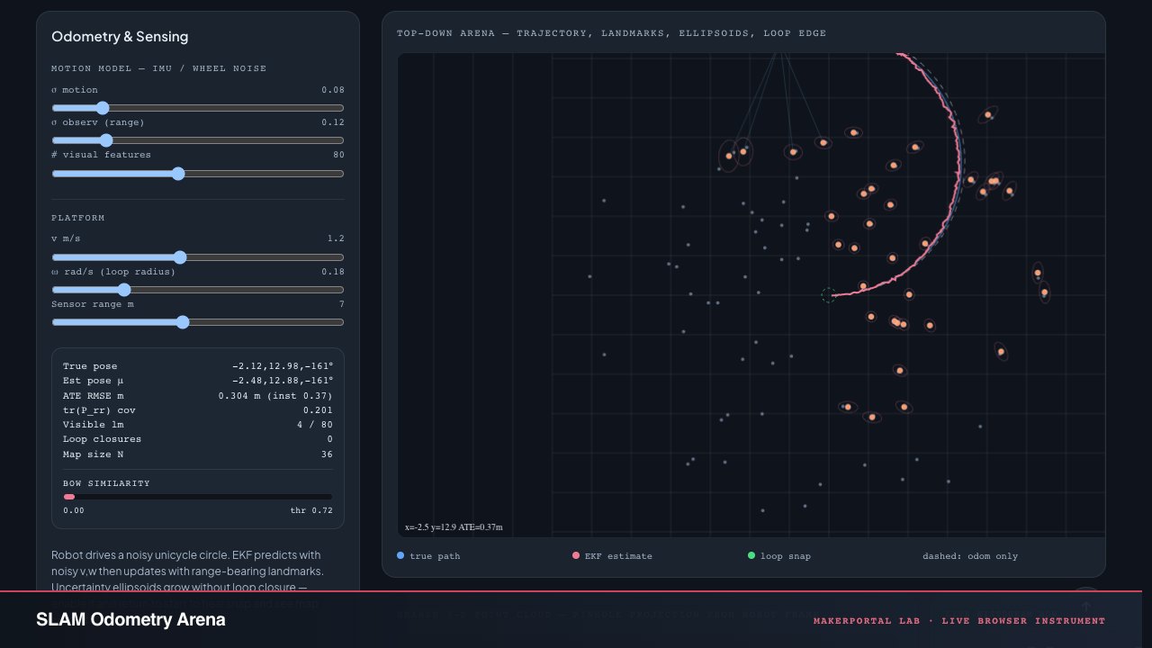
Continue the experiment