Playground · research instrument

Quantum Tunneling Simulator

Fire a Gaussian wave packet at a potential barrier and watch the wavefunction do what particles cannot: split into a reflected lobe and a transmitted one that leaked straight through a wall it did not have the energy to climb. The 1D time-dependent Schrödinger equation is integrated with the unitary Crank–Nicolson scheme, and the live transmission probability is checked against the exact barrier formula.

Independent research instrument — not claimed as MakerPortal shipped product code. Methods, equations, assumptions, and limitations are disclosed so you can inspect what the page does and does not establish.

Barrier & packet

Barrier height V₀5.0Barrier width3.0Packet momentum k₀3.0Packet width σ4.0

packet energy E = k₀²/2
4.50

regime
tunneling

Hardware hook:Get the Young’s Double-Slit Interference Kit (Laser) ↗

|ψ(x)|² & potential V(x)

t = 0.0 · norm = 1.000

Reflected (left of barrier)

—

Inside barrier

—

Transmitted (right)

—

Exact T (plane wave)

—

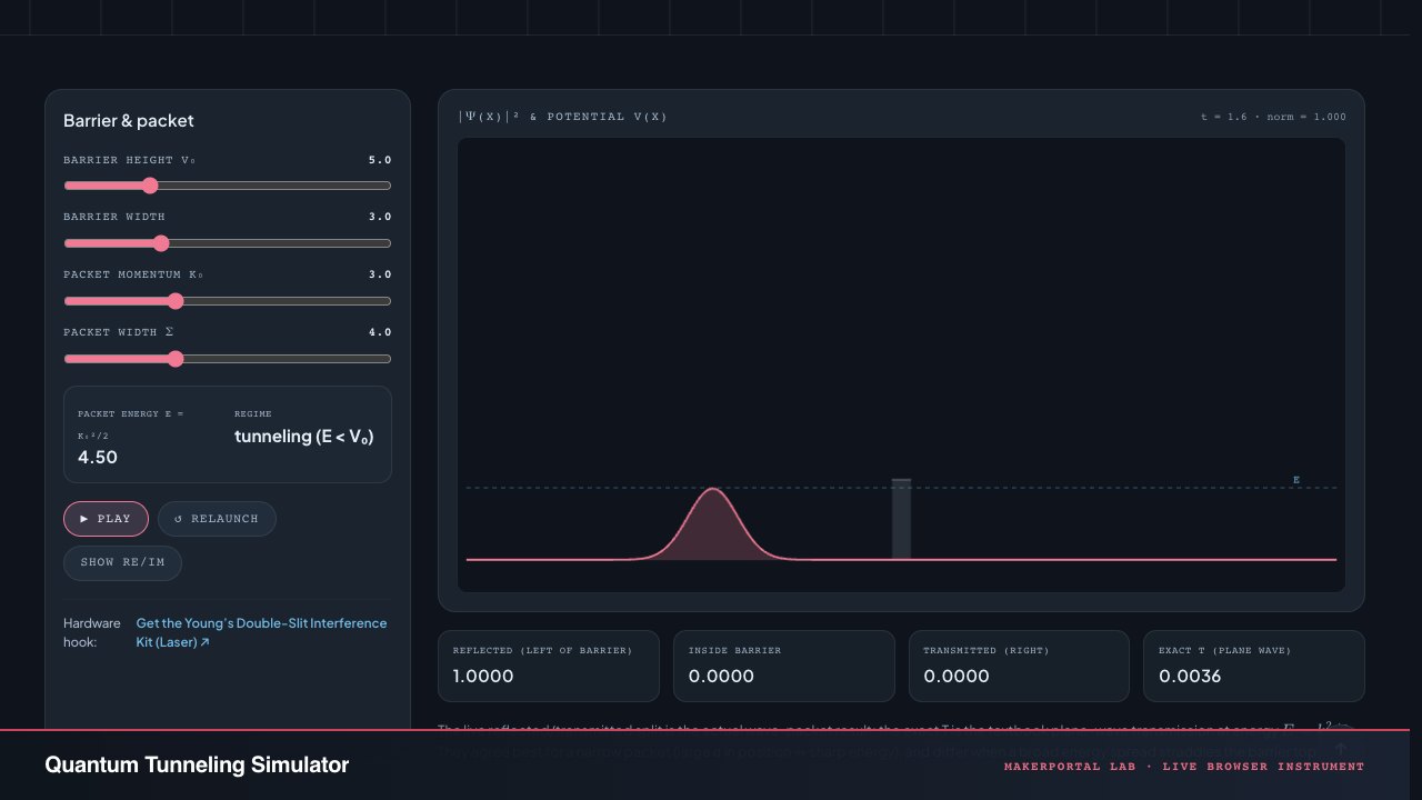
The live reflected/transmitted split is the actual wave-packet result; the exact T is the textbook plane-wave transmission at energy $E = k_0^2/2$ . They agree best for a narrow packet (large σ in position ⇒ sharp energy), and differ when a broad energy spread straddles the barrier top.

Anatomy of the instrument

Every pixel on the canvas answers to the physics below. Here is what each visual element and control is actually doing, and why it is built that way.

The wavefunction canvas

01
The $|\psi|^2$ filled area. Probability density encoded as a filled translucent region under the waveform envelope. The brighter the fill, the more likely the particle is found at that position. The upper stroke traces the density outline — peak height is the most probable location.
02
The potential barrier rectangle. A semi-transparent box spanning the barrier width at the scaled $V_0$ height. The horizontal energy dashed line (anchor blue) sits at $E = k_0^2/2$ and visually answers the central question: is the particle energy above or below the barrier?
03
The Re/Im toggle overlay. When enabled, two faint waveforms — blue for $\operatorname{Re}(\psi)$ and pink for $\operatorname{Im}(\psi)$ — are drawn behind the probability density. Their relative phase encodes the local momentum: crest-aligned means moving right, crest-opposed means moving left. The primary diagnostic for interference patterns.
04
Absorbing boundary layers. Quadratic imaginary-potential wells at the $[-70, -56]$ and $[56, 70]$ domain edges silently damp incoming amplitude. The wavefunction never sees a hard wall — it fades into the absorber instead, preventing the spurious reflections that would otherwise corrupt the transmitted and reflected readouts.
05
The render loop. Every frame advances 4 Crank–Nicolson steps ( $\Delta t = 0.02$ each, so 0.08 time units per frame). Every 25 frames the vertical scale auto-adjusts via a smooth lerp so the wavefunction always fills ~62% of the canvas height, preventing it from flattening as it spreads or shrinking as the absorber eats amplitude.

Tridiagonal system solved every step — Thomas algorithm, O(N)

b_j\psi_j^{n+1} + a\psi_{j-1}^{n+1} + a\psi_{j+1}^{n+1} = d_j

For each interior grid point $j = 1,\ldots, N-2$ , with $a = -\frac{i\Delta t}{4(\Delta x)^2}$ , $b_j = 1 + \frac{i\Delta t}{2}\bigl(\frac{1}{(\Delta x)^2} + V_j\bigr)$ , and RHS $d_j = \bigl[(I - \frac{i\Delta t}{2}H)\psi^n\bigr]_j$ . The matrix is tridiagonal because the kinetic operator couples only nearest neighbors. The Thomas algorithm solves it exactly in one forward sweep and one backward sweep — precisely two passes over the grid, no iteration, no matrix inversion.

Controls, readouts, and physics

01
Sliders. Four controls: barrier height $V_0$ (0–20), barrier width (0.2–10), packet momentum $k_0$ (0.5–8), and packet width $\sigma$ (1–10). Each slider input rebuilds the potential, re-initializes the wavefunction from $x_0 = -35$ , and restarts the clock.
02
Physics regime label. Computed live: $E = k_0^2/2$ . If $E < V_0$ the label reads "tunneling (E < V₀)", if $E > V_0$ it reads "over-barrier (E > V₀)", and at equality it reads "at barrier top". This is the regime switch between exponential decay inside the barrier and resonant transmission above it.
03
Readout cards. Four live numbers: Reflected ( $\int_{-\infty}^{w/2}|\psi|^2 dx$ left of the barrier), Inside barrier (within the walls), Transmitted (right of the barrier), and Exact T (the textbook plane-wave formula at energy E). The live and exact values converge for narrow packets in momentum space, and diverge when a broad energy spread straddles the barrier top.
04
Auto-rescale viewport. The $|\psi|^2$ peak is tracked every frame and the vertical scale factor $\alpha$ is lerped toward keeping it at 62% of the canvas height. The smooth factor (15% per rescale tick, every 25 frames) prevents jarring jumps while preventing the waveform from disappearing as it spreads or the absorber eats amplitude.
05
Play / Pause / Relaunch / Re/Im. Play toggles the animation loop. Relaunch resets the wavefunction and re-reads all slider values — the equivalent of setting up a new experiment. Show Re/Im overlays the real (blue) and imaginary (pink) parts of $\psi$ behind the probability density, revealing the phase structure that $|\psi|^2$ alone hides.

Gear behind this build

Quantum mechanics stack · 4 picks

Quantum hardware4

$49.99Book

Introduction to Quantum Mechanics

Chapters 2-3 cover time-independent Schrödinger equation, rectangular barrier, and exact transmission T = [1 + V0² sinh²(kL)/4E(V0-E)]⁻¹ that this Crank-Nicolson run checks live.

$49.99 USDView ↗

$62.86Book

Modern Quantum Mechanics

Chapter 2 solves barrier penetration via WKB and exact matching — launch a Gaussian packet in this page and compare measured T/R against Sakurai's analytic formula.

$62.86 USDView ↗

$57.30Book

Principles of Quantum Mechanics, 2nd Edition

Derives unitary evolution and Crank-Nicolson as Cayley form (I - iHΔt/2)/(I + iHΔt/2) preserving norm — the method this simulator uses for wave-packet tunneling.

$57.30 USDView ↗

$Young's Double-Slit Experiment, Single Slit, with Holder Observation Board Red Light Source, Optics Elements, Optical Physical Experiment Kit, Interference Diffraction Grating Sheet 50 * 50mm$ $25.98Kit

Young's Double-Slit Experiment, Single Slit, with Holder Observation Board Red Light Source, Optics Elements, Optical Physical Experiment Kit, Interference Diffraction Grating Sheet 50 * 50mm

Physical demonstration of matter-wave interference underlying Schrödinger's equation — same wave-particle duality that makes tunneling through a classically forbidden barrier possible.

$25.98 USDView ↗

Prices shown were retrieved from the Amazon Product Advertising API on 19 July 2026 and are indicative only — the price and availability on Amazon at the time of purchase apply.

More gear across every app: the full Gear list →

Method & limitations

We solve $i\frac{\partial\psi}{\partial t} = \bigl(-\frac{1}{2}\frac{\partial^2}{\partial x^2} + V\bigr)\psi$ in natural units ( $\hbar = m = 1$ ) on a uniform grid. Crank–Nicolson advances $(I + i\frac{\Delta t}{2}H)\psi^{n+1} = (I - i\frac{\Delta t}{2}H)\psi^n$ — the Cayley approximation to the exact propagator $e^{-iH\Delta t}$ . Because that operator is unitary, $\int|\psi|^2 dx$ is conserved to machine precision; each step is a tridiagonal complex solve via the Thomas algorithm. A thin imaginary (absorbing) potential at the domain edges soaks up outgoing amplitude so the walls do not reflect it back.

Time-dependent Schrödinger equation (ħ = m = 1)

i\frac{\partial\psi}{\partial t} = \left(-\frac{1}{2}\frac{\partial^2}{\partial x^2} + V(x)\right)\psi

In natural units the de Broglie wavelength is $\lambda = 2\pi/k$ , so $k_0 = 3$ corresponds to $\lambda \approx 2.1$ — well resolved on the $\Delta x \approx 0.14$ grid.

Crank–Nicolson propagator (Cayley form)

(I + \frac{i\Delta t}{2}H)\psi^{n+1} = (I - \frac{i\Delta t}{2}H)\psi^n

Unitary to machine precision: $\|\psi^{n+1}\| = \|\psi^n\|$ for real $V$ . Unconditionally stable — no CFL constraint on $\Delta t$ , unlike explicit schemes that blow up unless $\Delta t < (\Delta x)^2$ .

Transmission coefficient — below barrier ( $E < V_0$ )

T = \frac{1}{1 + \frac{V_0^2\sinh^2(\kappa w)}{4E(V_0 - E)}},\qquad \kappa = \sqrt{2(V_0 - E)}

Exponential decay inside the barrier: $\psi \propto e^{-\kappa x}$ . For $\kappa w \gg 1$ (wide/tall barrier), $T \approx \frac{16E(V_0-E)}{V_0^2}e^{-2\kappa w}$ — the classic Gamow factor.

Transmission coefficient — above barrier ( $E > V_0$ )

T = \frac{1}{1 + \frac{V_0^2\sin^2(k_2 w)}{4E(E - V_0)}},\qquad k_2 = \sqrt{2(E - V_0)}

Resonant transmission at $T = 1$ when $k_2 w = n\pi$ — the barrier acts as a Fabry–Pérot etalon. Between resonances the transmission dips but never vanishes.

Numerical parameters

$N = 1000$ grid points on domain $[-70, 70]$ with $\Delta x = 140/999 \approx 0.1401$ . Time step $\Delta t = 0.02$ . Four Crank–Nicolson steps per animation frame (× requestAnimationFrame at ≈ 60 Hz) gives ~5 seconds of simulated physics per wall-clock second. The absorbing boundary uses quadratic imaginary-potential caps $V_{\text{im}} = -2.5 f^2$ over the outermost 14 units on each side.

What is faithful

The full time-dependent Schrödinger dynamics — dispersion, interference, exponential decay inside the barrier, and the reflected/transmitted split — are all real, not cartooned. Unitarity is verified by unit test over hundreds of steps.

What it simplifies

One particle, one dimension, non-relativistic, on a finite grid. The absorbing layer trades a little exactness near the edges for the absence of wall reflections. No spin, no many-body correlations, no 2D/3D scattering.

The solver lives in src/lib/quantum.ts (Crank–Nicolson stepper, complex Thomas solver, exact rectangular-barrier transmission), unit-tested for norm conservation and the analytic transmission limits.

Two gotchas worth knowing

Absorbing boundaries eat probability

The quadratic imaginary-potential caps at the domain edges ( $V_{\text{im}}(x) = -2.5f^2$ , where $f = (d_{\text{edge}} - |x - x_{\text{wall}}|)/d_{\text{edge}}$ with $d_{\text{edge}} = 14$ ) deliberately leak amplitude to suppress wall reflections. The norm readout shows the drift — it starts at 1.000 and gradually falls. Keep runs under ~2000 time steps for a norm above 0.99. Longer runs see the wavefunction visibly shrink as the absorbers consume it from both ends.

$E \approx V_0$ resonance

When the packet energy sits exactly at the barrier height, the exact T formulas for $E < V_0$ and $E > V_0$ both approach a removable singularity — $\sinh(\kappa w) \to \kappa w$ and $\sin(k_2 w) \to k_2 w$ as $\kappa, k_2 \to 0$ . The code handles this with a separate limit branch ( $T = 1/(1 + V_0^2 w^2/(2E))$ ), but the numerical wave-packet dynamics at this boundary are sensitive: even a small energy spread puts part of the packet above and part below the barrier, so the live split and the exact formula can disagree more than usual.

TypeScript — the Crank–Nicolson stepper

The full solver lives in src/lib/quantum.ts. Here is the core class and the exact transmission formula — pure functions with zero dependencies beyond a Float64Array.

CrankNicolson1D + rectangularBarrierTransmission

export class CrankNicolson1D {
  readonly n: number;
  readonly dx: number;
  readonly dt: number;
  psi: ComplexArray;

  constructor(x: Float64Array, dt: number, Vre: Float64Array, Vim?: Float64Array) {
    this.n = x.length;
    this.dx = x[1] - x[0];
    this.dt = dt;
    this.Vre = Vre;
    this.Vim = Vim ?? new Float64Array(this.n);
    this.psi = { re: new Float64Array(this.n), im: new Float64Array(this.n) };
    // LHS off-diagonal: a = −i·dt/(4 dx²) — constant, symmetric
    this.aRe = 0;
    this.aIm = -this.dt / (4 * this.dx * this.dx);
    // Precompute LHS main diagonal b_j = 1 + i·dt/2·(1/dx² + V_j)
    this.bRe = new Float64Array(this.n - 2);
    this.bIm = new Float64Array(this.n - 2);
    for (let j = 0; j < this.n - 2; j++) {
      const diagKin = 1 / (this.dx * this.dx);
      this.bRe[j] = 1 + (this.dt / 2) * -this.Vim[j + 1];
      this.bIm[j] = (this.dt / 2) * (diagKin + this.Vre[j + 1]);
    }
  }

  step(): void {
    // Build RHS d = (I − i·dt/2 H) ψ^n over interior nodes
    const dRe = new Float64Array(this.n - 2);
    const dIm = new Float64Array(this.n - 2);
    for (let j = 1; j <= this.n - 2; j++) {
      const hRe = 1/this.dx**2 + this.Vre[j];
      const hIm = this.Vim[j];
      const mRe = 1 + (this.dt / 2) * hIm;
      const mIm = -(this.dt / 2) * hRe;
      let rr = mRe * this.psi.re[j] - mIm * this.psi.im[j];
      let ii = mRe * this.psi.im[j] + mIm * this.psi.re[j];
      const off = this.dt / (4 * this.dx * this.dx);
      rr += -off * (this.psi.im[j-1] + this.psi.im[j+1]);
      ii +=  off * (this.psi.re[j-1] + this.psi.re[j+1]);
      dRe[j-1] = rr;
      dIm[j-1] = ii;
    }
    // Thomas algorithm — O(N), no matrix inversion
    const sol = thomasSolveComplex(
      this.aRe, this.aIm, this.bRe, this.bIm,
      this.aRe, this.aIm, dRe, dIm
    );
    for (let j = 1; j <= this.n - 2; j++) {
      this.psi.re[j] = sol.re[j - 1];
      this.psi.im[j] = sol.im[j - 1];
    }
    this.psi.re[0] = this.psi.im[0] = 0;
    this.psi.re[this.n - 1] = this.psi.im[this.n - 1] = 0;
  }
}

export function rectangularBarrierTransmission(
  E: number, V0: number, L: number
): number {
  if (E <= 0) return 0;
  if (V0 <= 0) return 1;
  // E ≈ V₀: removable singularity — use limit form
  if (Math.abs(E - V0) < 1e-9 * Math.max(1, V0))
    return 1 / (1 + (V0**2 * L**2) / (2 * E));
  if (E < V0) {
    const kappa = Math.sqrt(2 * (V0 - E));
    const s = Math.sinh(kappa * L);
    return 1 / (1 + (V0**2 * s**2) / (4 * E * (V0 - E)));
  }
  const k2 = Math.sqrt(2 * (E - V0));
  const s = Math.sin(k2 * L);
  return 1 / (1 + (V0**2 * s**2) / (4 * E * (E - V0)));
}

Frequently asked questions

What is quantum tunneling?

A quantum particle has a nonzero chance of passing through a potential barrier even when its energy is below the barrier height — something impossible in classical mechanics. Its wavefunction decays exponentially inside the barrier rather than stopping, so a small but real amplitude leaks out the far side. It is the mechanism behind alpha decay, the scanning tunneling microscope, and tunnel diodes.

Why use the Crank–Nicolson method?

Crank–Nicolson is the Cayley form of the quantum propagator: it is unitary to machine precision, so total probability is conserved exactly for a real potential, and it is unconditionally stable, so it does not blow up the way a naive explicit scheme does. Each step solves a tridiagonal complex linear system with the Thomas algorithm, which is fast and exact.

Why does the transmission probability oscillate as I raise the energy above the barrier?

Above the barrier the particle is not guaranteed to pass — the barrier edges act like a thin film, and the transmitted amplitude interferes with itself. At energies where the barrier width is a half-integer number of wavelengths the transmission hits 100% (resonant transmission); between those it dips. The live number tracks the exact rectangular-barrier formula.

How is probability normalization maintained?

The Crank–Nicolson scheme is unitary to machine precision for a real potential — each step preserves ∫|ψ|² dx exactly. However, the absorbing boundary layers at the domain edges use a negative imaginary potential that deliberately removes amplitude, so total norm drifts slowly downward from 1. The simulation rescales the |ψ|² vertical axis every 25 frames to keep the waveform visible, and the norm readout shows the current total live so you can gauge how much has leaked into the absorbers.

Why are absorbing boundaries needed and how do they work?

The spatial domain is finite with Dirichlet walls (ψ = 0 at x = ±70). Without absorbing layers, any amplitude that reaches the edge reflects back inward, contaminating the transmitted and reflected signals. Quadratic imaginary-potential wells near both edges gradually damp the wavefunction before it hits the hard wall, suppressing reflections at the cost of slowly eroding total probability. Practical runs should stay under ~2000 time steps to keep the norm above 0.99.

Shareable still

The instrument, captured—not illustrated.

This 16:9 frame is rendered from the real browser instrument above. It is the page's canonical preview for image search, link unfurls, and posts that need to show what the tool actually does.

Download 1280 × 720 JPEG

Quantum Tunneling Simulator — live MakerPortal instrument screenshot — Canonical capture · real UI · no generated scientific artwork

Continue the experiment

All lab instruments →

Research

Quantum Tunneling Simulator

Barrier & packet

Anatomy of the instrument

The wavefunction canvas

Controls, readouts, and physics

Gear behind this build

Quantum hardware4

Introduction to Quantum Mechanics

Modern Quantum Mechanics

Principles of Quantum Mechanics, 2nd Edition

Young's Double-Slit Experiment, Single Slit, with Holder Observation Board Red Light Source, Optics Elements, Optical Physical Experiment Kit, Interference Diffraction Grating Sheet 50 * 50mm

Method & limitations

Two gotchas worth knowing

TypeScript — the Crank–Nicolson stepper

Frequently asked questions

The instrument, captured—not illustrated.

Live Earth

Double Pendulum + Phase Space

Chladni Cymatics

Quantum Tunneling Simulator

Tunneling simulator

Barrier & packet

Anatomy of the instrument

The wavefunction canvas

Controls, readouts, and physics

Gear behind this build

Quantum hardware4

Introduction to Quantum Mechanics

Modern Quantum Mechanics

Principles of Quantum Mechanics, 2nd Edition

Young's Double-Slit Experiment, Single Slit, with Holder Observation Board Red Light Source, Optics Elements, Optical Physical Experiment Kit, Interference Diffraction Grating Sheet 50 * 50mm

Method & limitations

Two gotchas worth knowing

TypeScript — the Crank–Nicolson stepper

Frequently asked questions

The instrument, captured—not illustrated.

Related instruments

Live Earth

Double Pendulum + Phase Space

Chladni Cymatics