Playground · research instrument

Magnetic Field Simulator

Every field line here is marched through 3D space by a 4th-order Runge–Kutta integrator following the exact Biot–Savart field of real current loops and wires. Switch between a single loop, a Helmholtz pair, a magnetic bottle, a solenoid, an antiparallel wire pair, and a bar-magnet dipole and watch the geometry of the field reorganize — the uniform core of a Helmholtz coil, the pinched mirrors of a bottle, the confined interior of a solenoid, the circulating wrapping of parallel wires.

Independent research instrument — not claimed as MakerPortal shipped product code. Methods, equations, assumptions, and limitations are disclosed so you can inspect what the page does and does not establish.

Live field-line tracer

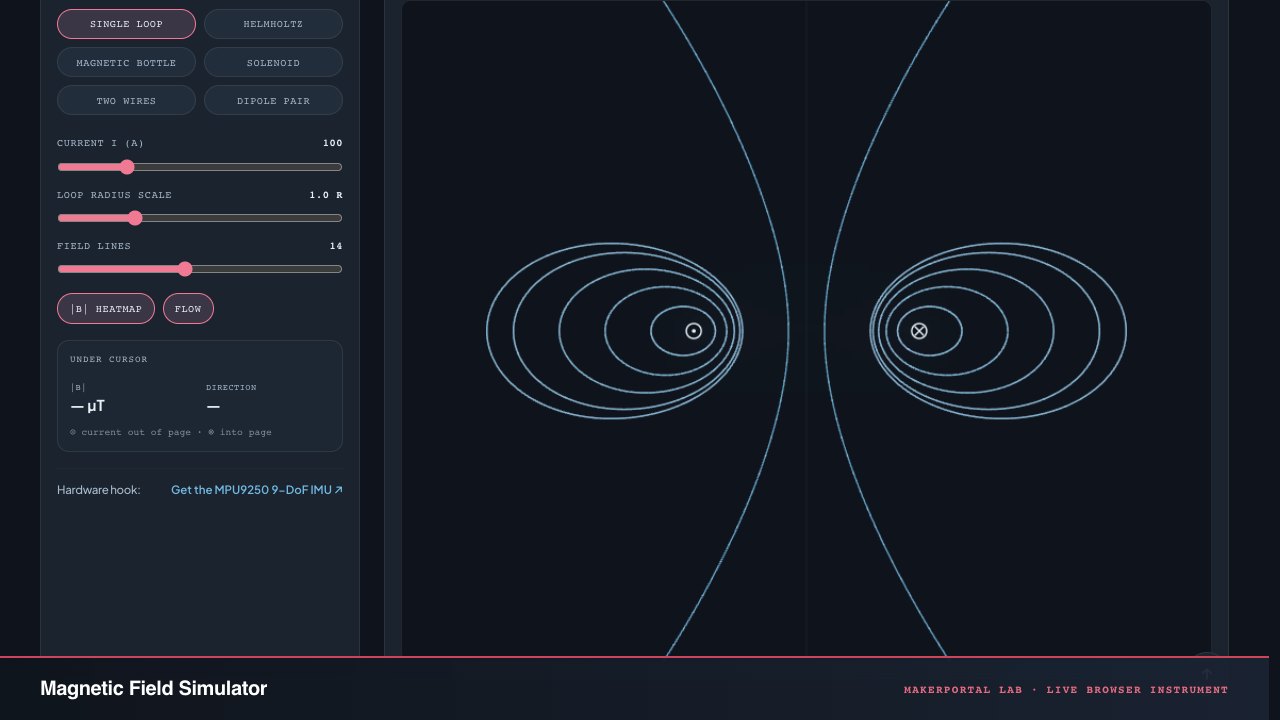
The canvas is a meridional cross-section through the symmetry axis of the current distribution: horizontal axis is $x$ (radial distance from the coil axis), vertical axis is $z$ (axial distance along the symmetry line). For coaxial configurations the magnetic field has zero out-of-plane $y$ -component in this plane, so every traced line stays exactly in-plane — no projection artifacts.

Configuration

Current I (A)100Coil separation1.0 RField lines14

Under cursor

|B|
— µT

direction
—

⊙ current out of page · ⊗ into page

Hardware hook:Get the MPU9250 9-DoF IMU ↗

Meridional cross-section (x–z plane)

axis of symmetry vertical

Anatomy of the instrument

Every pixel above answers to the math below. Here is what each piece of the visualization and every control is actually doing, and why it is built that way.

The field-line canvas

01
The coordinate geometry. The canvas shows the $x$ – $z$ plane through the symmetry axis of the current distribution. $x$ (horizontal) is the radial distance from the axis; $z$ (vertical) is the axial coordinate. For coaxial loop configurations the field $\mathbf{B}(x,0,z)$ has zero $y$ -component by azimuthal symmetry, so field lines traced in this plane stay in this plane — no projection artifacts, no 3D ambiguity.
02
The vertical dashed axis. The dashed line at $x=0$ is the symmetry axis — it passes through the centers of all coaxial loops. On this axis the field is purely vertical. The heatmap and field-line color encodes $|\mathbf{B}|$ on a logarithmic scale from the anchor blue (weak field) to the brand red (strong field). The color map is anchored at the 92nd-percentile field strength to avoid a single hotspot washing out the entire dynamic range.
03
The current glyphs. Each wire piercing the cross-section plane is marked by a circle: a filled dot ⊙ for current coming out of the page (toward you, +y), and a crossed circle ⊗ for current going into the page. The right-hand rule ties the glyph to the field circulation: with current out of the page at $+x$ on the axis, the field lines wrap counterclockwise.
04
Flow-direction dashes. A dashed stroke overlay animates along the traced field lines to show direction. The dash offset advances by 0.6 px per frame at 60 fps, giving a gentle 6-second loop cycle. The animation is driven by requestAnimationFrame only when the flow toggle is on and the page is visible — idle when hidden or toggled off. The reduces-motion OS preference pauses the animation entirely.
05
The heatmap. The $|\mathbf{B}|$ magnitude is evaluated on a grid (down to 5 px cells, auto-coarsened to 8 or 12 if the initial pass exceeds 8 ms) using compiledFieldAt — the same zero-allocation Struct-of-Arrays evaluator the field lines use. The heatmap is computed once per scene rebuild (not per frame) and cached to an offscreen canvas. Switching it off skips both evaluation and blit.

What every traced line satisfies — dr/ds = B̂(r)

\frac{d\mathbf{r}}{ds} = \hat{\mathbf{B}}(\mathbf{r}) = \frac{\mathbf{B}(\mathbf{r})}{|\mathbf{B}(\mathbf{r})|}

A field line is a curve whose tangent vector at every point is parallel to $\mathbf{B}$ . The RK4 integrator steps along the unit field direction at constant arclength $ds = 5\ \text{mm}$ , using 4 field evaluations per step. The arclength is fixed so lines in weak-field regions don't take huge leaps — field magnitude is encoded by line density and color, not step size.

Controls, readouts, and render loop

01
Preset buttons. Six configurations: single loop (a pure dipole), Helmholtz pair (two coplanar loops at $s=R$ spacing for uniform field), magnetic bottle (anti-Helmholtz: opposite currents create the mirror geometry), solenoid (3–12 turns creating a confined interior), two antiparallel wires (circulating field around each), and a dipole pair (coaxial loops at variable separation, approximating a bar magnet).
02
Current slider (10–400 A). Scales the field magnitude linearly. $\mathbf{B} \propto I$ in DC magnetostatics — doubling the current doubles every field value everywhere. The loop radius is fixed at $R = 0.1\ \text{m}$ , so the on-axis dipole field at the loop center is $B = \mu_0 I / (2R)$ .
03
Geometry slider. Separation between loops in units of the loop radius $R$ . At $s/R = 1.0$ , two coaxial same-current loops form the Helmholtz condition — second derivative of $B_z$ vanishes on axis, producing the flattest possible central field. For the solenoid preset this slider controls the number of turns instead of separation.
04
Field-line count (6–24). Seeds are placed along the $x$ -axis at equally spaced radial distances from the loop center, half in each direction. Each seed is traced both forward and backward along $\pm\hat{\mathbf{B}}$ , then joined into a single polyline. Lines with fewer than 4 points are discarded — these are seeds that land inside a loop or too close to a wire axis.
05
Cursor readout. Moving the mouse over the canvas evaluates compiledFieldAt at the mapped physical coordinate and reports $|\mathbf{B}|$ in $\mu\text{T}$ (or $\text{mT}$ above 1000 µT) and the field direction angle relative to the horizontal. This is the same solver used by the field lines and heatmap — a single source of truth.
06
The render loop. There is no idle requestAnimationFrame spin. The scene rebuilds (segment compilation, field-line tracing, heatmap, cached layer draw) only on parameter change. The flow-direction dashes run an independent rAF loop that pauses when the canvas is offscreen (IntersectionObserver) or the page is hidden (visibilitychange). State changes issue a single draw() call — no wasted frames while you read.

Gear behind this build

Magnetostatics hardware · 7 picks

Magnetic-field sensing7

$43.99Sensor

EC Buying GY-MPU9250 9 Axis Sensor 9 DOF Accelerometer with Gyroscope and Magnetic Field Sensors, 16 Bit AD Converter Data Output IIC I2C SPI

9-DoF IMU used in BLExAR's calibration builds. The onboard magnetometer is a 3-axis Hall-effect sensor — the same physics modeled by the magnetic field-line tracer — while the DMP outputs attitude as a quaternion matching CMHeadphoneMotionManager's format.

$43.99 USDView ↗

$11.99Tool

Green Magnetic Viewing Film 4x6 | Cool Magnets Science Kit | Magnetic Field Detector & Visual Aid for Physics Education | Ideal for Research & Magnetism Demonstrations

Shows Helmholtz pair uniformity and solenoid fringe fields in real life — directly comparable to the B_z magnitude readout under your cursor.

$11.99 USDView ↗

$18.01Tool

Magnetic Field Viewing Film, Magnetic Field Viewer, 4 x 4 Inch

Green film renders flux lines from Biot-Savart superposition visible — lay it over a current loop and see the same dipole field this simulator traces via Runge-Kutta.

$18.01 USDView ↗

$18.99Sensor

GREDIA 3/4" Water Flow Sensor Food-Grade Switch Hall Effect Flowmeter Fluid Meter Counter 1-60L/min (Pack of 2）

Flow sensor used in BLExAR's water-metering build. Uses a Hall-effect magnetic sensor — the same Biot–Savart field the tracer models.

$18.99 USDView ↗

$49.18Book

Introduction to Electrodynamics

Chapter 5 derives Biot-Savart law and Helmholtz coil field — the exact integral this tracer evaluates with RK4 field-line marching.

$49.18 USDView ↗

$72.19Sensor

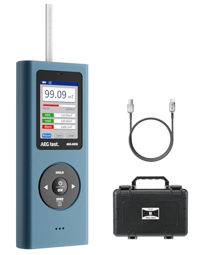
AEGTEST 8035 DC Gauss Meter, Telescopic Hall Sensor, Rechargeable Tesla Meter 0–2500 mT, Magnetometer with Data Logging and Alarm, Magnetic Field Strength Meter, ±5% General Accuracy for Daily Use

Measures B-field magnitude around loops/solenoids — hand-verify the Biot-Savart μ0/4π scaling this tracer computes before field-line integration.

$72.19 USDView ↗

$21.98Apparatus

Ferrofluid Magnetic Display – Science Education Magnetism Kit – Interactive Liquid Metal Physics Demonstration – Executive Desk Décor with Neodymium Magnets – STEM Learning Tool

Ferrofluid spikes under magnetic field emulate ferrofluid cooling in voice-coil gaps — the same thermal-magnetic mechanism reducing thermal compression via enhanced heat transfer.

$21.98 USDView ↗

Prices shown were retrieved from the Amazon Product Advertising API on 19 July 2026 and are indicative only — the price and availability on Amazon at the time of purchase apply.

More gear across every app: the full Gear list →

The math and physics, in full

From the Biot–Savart law through the finite-segment closed form to the RK4 integration — every equation this tracer evaluates, with the discretization choices and error bounds made explicit.

The Biot–Savart law, finite-segment form

In DC magnetostatics a steady current $I$ flowing through a wire produces a magnetic field at observation point $\mathbf{P}$ . The differential form sums contributions from each infinitesimal length $d\mathbf{l}$ :

Differential Biot–Savart

d\mathbf{B} = \frac{\mu_0 I}{4\pi} \frac{d\mathbf{l} \times \hat{\mathbf{r}}}{r^2}

Integrating $d\mathbf{B}$ around a closed loop gives the total field. For a straight wire segment from $A$ to $B$ the integral has a closed form. Let $d$ be the perpendicular distance from the wire line to $\mathbf{P}$ , $\hat{\mathbf{e}}$ the unit vector along the wire (current direction), $\hat{\mathbf{n}}$ the unit vector from the wire line to $\mathbf{P}$ , and $\theta_1, \theta_2$ the angles the wire endpoints subtend:

Finite-segment closed form

\mathbf{B} = \frac{\mu_0 I}{4\pi d} (\cos\theta_1 - \cos\theta_2) (\hat{\mathbf{e}} \times \hat{\mathbf{n}})

Implemented as segmentField() in src/lib/emfields.ts. The denominator $d$ is clamped at $10^{-9}\ \text{m}$ to avoid the wire-axis singularity. In the limit $\ell \to \infty$ with $\cos\theta_1 \to 1, \cos\theta_2 \to -1$ this recovers the familiar infinite-wire result $\mathbf{B} = \mu_0 I / (2\pi d)$ .

A circular loop is approximated by $n_{\text{seg}} = 96$ straight chords. The chord approximation error scales as $\mathcal{O}(1/n_{\text{seg}}^2)$ for the field at distances comparable to the loop radius — 96 segments gives sub-pixel accuracy at the canvas scale. The total field at any point is the superposition (simple vector sum) of every segment's contribution.

Field-line integration: RK4

A magnetic field line satisfies the first-order ODE:

\frac{d\mathbf{r}}{ds} = \hat{\mathbf{B}}(\mathbf{r})

The field is renormalized at every step. A field line follows $\mathbf{B}$ 's direction but not its magnitude — the magnitude encodes the local field strength, not the geometry of the line. Integrating the raw $\mathbf{B}$ (unnormalized) would take giant steps in strong-field regions and tiny ones in weak regions, not a reflection of the actual curve geometry.

We integrate with classical 4th-order Runge–Kutta at fixed arclength step $h = 0.005\ \text{m}$ :

Classical RK4 weights

\begin{aligned} \mathbf{k}_1 &= h\,\hat{\mathbf{B}}(\mathbf{r}_n) \\ \mathbf{k}_2 &= h\,\hat{\mathbf{B}}(\mathbf{r}_n + \tfrac{1}{2}\mathbf{k}_1) \\ \mathbf{k}_3 &= h\,\hat{\mathbf{B}}(\mathbf{r}_n + \tfrac{1}{2}\mathbf{k}_2) \\ \mathbf{k}_4 &= h\,\hat{\mathbf{B}}(\mathbf{r}_n + \mathbf{k}_3) \\ \mathbf{r}_{n+1} &= \mathbf{r}_n + \tfrac{1}{6}(\mathbf{k}_1 + 2\mathbf{k}_2 + 2\mathbf{k}_3 + \mathbf{k}_4) \end{aligned}

Global truncation error is $\mathcal{O}(h^4)$ . At 5 mm step size over a typical half-line of 500 steps (2.5 m physical arclength), the accumulated geometric error is under 0.1 mm — well below one canvas pixel (~0.9 mm physical). Each step evaluates compiledFieldAt 4 times (once per stage).

Each seed is traced in both forward ( $+\hat{\mathbf{B}}$ ) and reverse ( $-\hat{\mathbf{B}}$ ) directions. Traces stop when $|\mathbf{B}|$ drops below $\mu_0 \times 10^{-4}\ \text{T}$ (fade-out in weak field), after 1100 steps (divergence guard), or when the line leaves the bounding box $|x|,|z| > 0.34\ \text{m}$ — all well beyond the canvas viewport.

Key configurations: when the math locks in

Helmholtz condition: s = R

\left.\frac{\partial B_z}{\partial z}\right|_{z=0} = 0,\quad \left.\frac{\partial^2 B_z}{\partial z^2}\right|_{z=0} = 0

Two coaxial loops spaced by exactly their radius cancel both first and second axial derivatives at the midpoint. The central field is $B = \left(\frac{4}{5}\right)^{3/2} \frac{\mu_0 I}{R}$ . The heatmap confirms this — the central region is uniformly tinted, no gradient visible.

On-axis loop field (verification formula)

B_z(z) = \frac{\mu_0 I R^2}{2(R^2 + z^2)^{3/2}}

This analytic formula is used as a unit-test oracle for fieldAt in emfields.ts. The chord-discretized field is verified to converge to this formula as $n_{\text{seg}} \to \infty$ .

Magnetic bottle: anti-Helmholtz

B_z(z) \propto z \quad\text{near } z=0

Opposite currents create a field that vanishes linearly at the midpoint and grows at both ends. The field-line geometry shows this as a pinch — lines converge at the strong-field ends and diverge in the weak center. Charged particles gyrate around the lines and reflect where the field strengthens (the magnetic mirror effect).

Long solenoid: ideal interior

B_{\text{interior}} \approx \mu_0 n I

For a solenoid with $n$ turns per meter and length $\ell \gg R$ , the interior field is nearly uniform and axial, with fringing at the ends. The tracer's solenoid preset stacks 3–12 loops along the axis — the interior field lines run parallel and evenly spaced, visually confirming the uniform-flux approximation.

Numerical method comparison

Method	Order	Evaluations / step	Error / step
Euler (naive)	1st	1	$\mathcal{O}(h^2)$
Midpoint (RK2)	2nd	2	$\mathcal{O}(h^3)$
Classical RK4 (used here)	4th	4	$\mathcal{O}(h^5)$ local, $\mathcal{O}(h^4)$ global

RK4 over Euler is not a tweak — it's the difference between a closed-loop field line and one that spirals into the canvas border after 200 steps. The 4x field evaluation cost per step is paid once per scene rebuild, not per frame, so it never blocks user interaction.

Three real-world traps

Chord discretization error

A 96-chord polygon approximating a circle has a perimeter that's 99.97% of the exact circumference. But the field inside the loop — within a few chord-lengths of the wire — is more sensitive. At grid points very close to a chord, the finite-segment formula sees a straight wire, not a curved one. The error is $\lesssim 0.1\%$ at one chord-length from the loop and vanishes rapidly with distance. If you need interior-field precision for a real coil design, use a higher segment count or a true elliptic-integral formula — this tracer prioritizes visual fidelity over engineering-grade precision.

Wire-axis singularity

The Biot–Savart formula blows up as $1/d$ when $d \to 0$ (on the wire axis). The solver clamps the perpendicular distance at $10^{-9}\ \text{m}$ , returning $\mathbf{0}$ for points closer than that. A real wire has finite radius — the field inside a cylindrical conductor grows linearly with $r$ from zero on the axis, not singular. This tracer treats wires as infinitely thin filaments, so the field near a glyph is capped, not physically accurate.

Seed placement bias

Field-line seeds are placed on the $x$ -axis only — no off-axis seeds, no adaptive density based on local $|\mathbf{B}|$ . This means lines in regions far from the axis (e.g., the return field of a solenoid) are sparser than they should be for true flux-area encoding. A production field-line tracer would seed adaptively — more seeds where $|\mathbf{B}|$ is high — but this adds complexity to collision detection (lines shouldn't cross) that we chose to defer.

The solver lives in src/lib/emfields.ts — unit-tested against the on-axis loop formula, the Helmholtz center value, and the circular field lines of a long straight wire.

Already know the coil? 210 solenoids are solved in advance →Centre field per amp-turn, the span each coil holds to within 1%, how far the µ0·n·I shortcut overstates it, and the turn count below which that shortcut stops being true.

The solver, in TypeScript

The finite-segment Biot–Savart evaluator and RK4 field-line tracer — the two functions that drive every pixel on this page. If you're porting this to C/C++ for an embedded magnetometer calibration tool, the logic ports directly.

Biot–Savart + RK4 tracer (TypeScript)

// Finite-segment Biot–Savart (src/lib/emfields.ts)
export function segmentField(seg: Segment, p: Vec3): Vec3 {
  const eVec = sub(seg.b, seg.a);
  const len = norm3(eVec);
  if (len < 1e-15) return [0, 0, 0];
  const e: Vec3 = scale(eVec, 1 / len);

  const aToP = sub(p, seg.a);
  const along = dot(aToP, e);
  const perp = sub(aToP, scale(e, along));
  let d = norm3(perp);
  if (d < 1e-9) return [0, 0, 0]; // on wire axis

  const nHat: Vec3 = scale(perp, 1 / d);
  const bToP = sub(p, seg.b);
  const ra = norm3(aToP);
  const rb = norm3(bToP);
  const cos1 = dot(aToP, e) / ra;
  const cos2 = dot(bToP, e) / rb;

  const mag = (MU0 * seg.current) / (4 * Math.PI * d) * (cos1 - cos2);
  return scale(cross(e, nHat), mag);
}

// RK4 field-line tracer — dr/ds = B̂(r)
export function traceFieldLine(
  cs: CompiledSegments, start: Vec3, opts: TraceOptions
): FieldLine {
  const h = opts.reverse ? -opts.step : opts.step;
  let p = start, k1 = null;

  for (let i = 0; i < opts.maxSteps; i++) {
    if (!k1) { const [d, ] = dir(p); if (!d) break; k1 = d; }
    const [k2, ] = dir(add(p, scale(k1, h/2)));
    if (!k2) break;
    const [k3, ] = dir(add(p, scale(k2, h/2)));
    if (!k3) break;
    const [k4, ] = dir(add(p, scale(k3, h)));
    if (!k4) break;
    p = add(p, scale([
      k1[0]+2*k2[0]+2*k3[0]+k4[0],
      k1[1]+2*k2[1]+2*k3[1]+k4[1],
      k1[2]+2*k2[2]+2*k3[2]+k4[2]
    ], h/6));
    points.push(p);
    const [nextK1, ] = dir(p);
    k1 = nextK1;
    if (Math.abs(p[0]) > bound || Math.abs(p[2]) > bound) break;
  }
}

Frequently asked questions

What is the Biot–Savart law?

It gives the magnetic field produced by a steady current: each infinitesimal length of current dl contributes a field dB proportional to I·dl × r̂ / r². Integrating over the whole circuit gives the total field at any point. Here every loop is broken into straight chords and each chord uses the exact finite-wire closed form, so the sum converges to the smooth loop as chord count grows.

Why use Runge–Kutta to draw field lines?

A field line is a curve everywhere tangent to B — mathematically, dr/ds = B̂(r). That is an ordinary differential equation. 4th-order RK4 integrates it with global truncation error O(h⁴), whereas naive Euler accumulates O(h) error per step and spirals field lines away from their true paths. The step size here is 5 mm per integration step, with up to 1100 steps per half-line, so the accumulated geometric error is well below one pixel.

What is a magnetic bottle?

Two coaxial coils carrying opposite currents (an anti-Helmholtz pair) create a field that is weak in the middle and strong at both ends. Charged particles spiralling along the lines get reflected at the high-field "mirrors" and bounce back and forth — the confinement principle behind magnetic-mirror fusion devices and the Van Allen radiation belts.

What does the Helmholtz spacing s = R do?

When two coaxial loops carrying the same current are spaced exactly one radius apart (s = R), the first and second spatial derivatives of B vanish at the midpoint. The result is a region of remarkably uniform magnetic field — the flattest possible for two coaxial coils. The on-axis midpoint field is B = (4/5)^(3/2) · μ₀ I / R.

What does this model leave out?

Pure DC magnetostatics: steady currents, filamentary (zero-thickness) wires, no magnetic materials (µ = µ₀ everywhere), no induced or eddy currents, no time variation. Loops are approximated by straight chords. It is exact for the idealised filamentary currents shown, but it is not a finite-element electromagnetic solver. Real-world effects like skin depth, wire thickness, and permeable cores are absent.

Shareable still

The instrument, captured—not illustrated.

This 16:9 frame is rendered from the real browser instrument above. It is the page's canonical preview for image search, link unfurls, and posts that need to show what the tool actually does.

Download 1280 × 720 JPEG

Magnetic Field Line Tracer — live MakerPortal instrument screenshot — Canonical capture · real UI · no generated scientific artwork

Continue the experiment

All lab instruments →

Research

Magnetic Field Simulator

Live field-line tracer

Configuration

Anatomy of the instrument

The field-line canvas

Controls, readouts, and render loop

Gear behind this build

Magnetic-field sensing7

EC Buying GY-MPU9250 9 Axis Sensor 9 DOF Accelerometer with Gyroscope and Magnetic Field Sensors, 16 Bit AD Converter Data Output IIC I2C SPI

Green Magnetic Viewing Film 4x6 | Cool Magnets Science Kit | Magnetic Field Detector & Visual Aid for Physics Education | Ideal for Research & Magnetism Demonstrations

Magnetic Field Viewing Film, Magnetic Field Viewer, 4 x 4 Inch

GREDIA 3/4" Water Flow Sensor Food-Grade Switch Hall Effect Flowmeter Fluid Meter Counter 1-60L/min (Pack of 2）

Introduction to Electrodynamics

AEGTEST 8035 DC Gauss Meter, Telescopic Hall Sensor, Rechargeable Tesla Meter 0–2500 mT, Magnetometer with Data Logging and Alarm, Magnetic Field Strength Meter, ±5% General Accuracy for Daily Use

Ferrofluid Magnetic Display – Science Education Magnetism Kit – Interactive Liquid Metal Physics Demonstration – Executive Desk Décor with Neodymium Magnets – STEM Learning Tool

The math and physics, in full

The Biot–Savart law, finite-segment form

Field-line integration: RK4

Key configurations: when the math locks in

Numerical method comparison

Three real-world traps

The solver, in TypeScript

Frequently asked questions

The instrument, captured—not illustrated.

Live Earth

Double Pendulum + Phase Space

Chladni Cymatics

Magnetic Field Simulator

Live field-line tracer

Configuration

Anatomy of the instrument

The field-line canvas

Controls, readouts, and render loop

Gear behind this build

Magnetic-field sensing7

EC Buying GY-MPU9250 9 Axis Sensor 9 DOF Accelerometer with Gyroscope and Magnetic Field Sensors, 16 Bit AD Converter Data Output IIC I2C SPI

Green Magnetic Viewing Film 4x6 | Cool Magnets Science Kit | Magnetic Field Detector & Visual Aid for Physics Education | Ideal for Research & Magnetism Demonstrations

Magnetic Field Viewing Film, Magnetic Field Viewer, 4 x 4 Inch

GREDIA 3/4" Water Flow Sensor Food-Grade Switch Hall Effect Flowmeter Fluid Meter Counter 1-60L/min (Pack of 2）

Introduction to Electrodynamics

AEGTEST 8035 DC Gauss Meter, Telescopic Hall Sensor, Rechargeable Tesla Meter 0–2500 mT, Magnetometer with Data Logging and Alarm, Magnetic Field Strength Meter, ±5% General Accuracy for Daily Use

Ferrofluid Magnetic Display – Science Education Magnetism Kit – Interactive Liquid Metal Physics Demonstration – Executive Desk Décor with Neodymium Magnets – STEM Learning Tool

The math and physics, in full

The Biot–Savart law, finite-segment form

Field-line integration: RK4

Key configurations: when the math locks in

Numerical method comparison

Three real-world traps

The solver, in TypeScript

Frequently asked questions

The instrument, captured—not illustrated.

Related instruments

Live Earth

Double Pendulum + Phase Space

Chladni Cymatics