Playground · research instrument

Conformal Map Viewer

A rectangular grid on the complex plane, warped live under f(z). Pick a preset or type your own expression in z, then drag the homotopy slider to morph continuously between the flat grid and its image.

Independent research instrument — not claimed as MakerPortal shipped product code. Methods, equations, assumptions, and limitations are disclosed so you can inspect what the page does and does not establish.

f(z)

PresetExpression (in z)

Supported: + - * / ^, parentheses, i, pi, e, and sin cos tan exp log sqrt conj abs of z. Parsed by a small hand-written evaluator — no eval.

Homotopy t0.00

t=0 is the flat grid, t=1 is the full image of f(z). p(t,z) = (1−t)·z + t·f(z).

Domain radius2.5Grid lines17

Complex plane

What "conformal" actually means

Put a tiny plus-sign + on the complex plane at some point $z_0$ . Push it through $f$ . If $f'(z_0) \neq 0$ , that plus stays a plus — maybe rotated, maybe scaled, but still $90^\circ$ . It does not shear into an X. That is conformity. Analytic functions with non-zero derivative are locally just rotation plus dilation. First order Taylor: $f(z) \approx f(z_0) + f'(z_0)(z - z_0)$ . Multiply by the complex number $f'(z_0)$ — that is argument rotation and magnitude stretch, nothing else.

When it holds — and why you see right angles

Condition is sharp: $f$ analytic and $f'(z_0) \neq 0$ . Then $f$ preserves oriented angles and local shapes. Your grid above is built from orthogonal lines $\text{Re} z = \text{const}$ and $\text{Im} z = \text{const}$ . Under any conformal $f$ , their images still intersect orthogonally wherever derivative does not vanish. Look at $e^z$ , $\sin z$ , Möbius — squares stay squares infinitesimally, even though globally they stretch wildly.

Picture it as $f$ having a local linear approximation that is a similarity: no squash. That is why conformal maps are the darling of fluid flow and electrostatics — if you understand flow around a circle, $f$ carries it to flow around anything $f(\text{circle})$ preserves.

When it fails — critical points

Where $f'(z)=0$ , conformality breaks. Angle doubles, triples, collapses. $f(z)=z^2$ has $f'(z)=2z$ , zero at origin. A $90^\circ$ crossing becomes $180^\circ$ — the grid forms a cusp. $z^3$ has $f'(z)=3z^2$ , so $90^\circ$ becomes $270^\circ$ at 0. In general, $f(z) \approx z^k$ multiplies angles by $k$ . That is not a rendering glitch; it is the map forgetting direction because leading term vanished.

The renderer shows this honestly. At the origin for $z^2$ , watch four right angles crush to two. At critical points you lose invertibility — locally many-to-one.

The slider

A homotopy, not physics

The $t$ -slider blends identity with $f$ : $p(t,z) = (1-t)z + t f(z)$ , $t \in [0,1]$ . $t=0$ flat grid, $t=1$ full image. For intermediate $t$ , $p$ is generally not conformal — it is an affine blend of two maps, not analytic composition. We use it to track where each line came from. That is why halfway, angles are not preserved. At $t=1$ they are, again modulo critical points.

p(0,z)=z

flat

p(t,z)=(1-t)z + t f(z)

blend

p(1,z)=f(z)

image

A field guide to the presets

Monomials $z^n$

$z^2, z^3$ . Critical point at 0 of order n-1. Angles multiply by $n$ , wraps plane $n$ times. Purest example of $f'(z)=0$ failure. Far from origin dominates — grows like $r^n$ .

Reciprocal 1/z

$f(z)=1/z$ . Pole at 0 — not a zero of derivative but infinity. Outside/inside swap, lines through origin become themselves. Möbius with $c \neq 0$ . Renderer clips when $|p| > \text{clamp}$ to avoid streaks to infinity. Those gaps are truth, not bug.

Exponential $\exp(z)$

$\exp(x+iy)=e^x (\cos y + i \sin y)$ . Vertical lines $x=\text{const}$ become circles radius $e^x$ , horizontal $y=\text{const}$ become rays angle $y$ . Periodic in $y$ with $2\pi$ . Never zero, $f' = f \neq 0$ , so conformal everywhere. Essential singularity at $\infty$ .

Möbius (z-1)/(z+1)

General form $\frac{a z + b}{c z + d}$ , $ad - bc \neq 0$ . Bijective on Riemann sphere, maps circles/lines to circles/lines. No critical points — $f' = (ad-bc)/(c z + d)^2 \neq 0$ . Automorphisms of sphere. Our example sends $1\to0$ , $-1\to\infty$ , $0\to-1$ .

Joukowski z + 1/z

Classic airfoils. $f(z)=z+1/z$ , $f'(z)=1-1/z^2$ , zero at $\pm1$ — where smooth circle maps to sharp trailing edge. That loss of conformality is the feature: it creates a cusp that Kutta condition needs. Unit circle maps to [-2,2] real segment.

$\sin z, \log z, \sqrt{z}$

$\sin z$ entire, $f'=\cos z$ zero at $\pi/2 + k\pi$ . $\log z$ not entire — branch cut, we take principal $\ln|z|+i \arg z$ . $\sqrt{z}$ two-valued; we pick principal branch. Both illustrate branch points: cannot be continuous on punctured plane without cut.

Poles vs zeros vs essential — how to read gaps

Pole: $|f(z)|\to\infty$ as $z\to z_0$ , near it behaves like $1/(z-z_0)^k$ . Grid lines explode outward, then re-enter from opposite direction. We detect $|\text{mapped}| > \text{view} \times 2.4$ or non-finite and lift pen. No line drawn to infinity — instead a gap. That gap location is the pole.

Zero: $f(z_0)=0$ . 1/z zero at $\infty$ , $z^2$ zero at 0. Locally angle-preserving unless also critical.

Essential: wilder than any pole, e.g. $e^z$ at $\infty$ , $\sin(1/z)$ near 0. Picard says it hits almost every value infinitely often in any neighborhood. In the plot you see infinite oscillation as you approach — again, not a bug, Picard in action.

Parser is hand-written recursive descent, no eval, complex arithmetic in plain ${\text{re},\text{im}}$ objects. Supports $+, -, \times, /, \hat{\phantom{x}}$ , $i, \pi, e$ , and $\sin, \cos, \tan, \exp, \log, \sqrt{\cdot}, \mathrm{conj}, \mathrm{abs}$ . Derivative-zero detection is left to your eyes — that is the point.

Anatomy of the instrument

Every pixel on that canvas answers to the math below. Here is what each piece of the visualization and controls is actually doing, and why it is built that way.

The conformal grid canvas

01
The Cartesian grid before transformation. A family of horizontal lines (fixed $\text{Im}\,z$ , rendered in blue/teal) and vertical lines (fixed $\text{Re}\,z$ , rendered in orange/red). At t=0, this is what you see: an ordinary rectangular lattice on $[-R,R]\times[-R,R]$ with a configurable number of lines set by the grid density slider.
02
How each grid point (x + iy) gets mapped via f(z). The script samples every grid line at 90 points, evaluates the parsed AST at each complex coordinate $z = x + iy$ , then blends with the identity via the homotopy $p(t,z) = (1-t)z + t f(z)$ . Each evaluated point goes through a clamp-radius check — if $|p| > \text{view} \times 2.4$ or if the result is non-finite, the pen lifts, creating a visible gap.
03
Color encoding. Horizontal grid lines (constant imaginary part) get a blue-family hue that shifts slightly per line — warmer toward positive imaginary values, cooler toward negative. Vertical lines (constant real part) get an orange/red-family hue, shading toward the positive real axis. The axis lines (where fixed component is near zero) are drawn with a slightly heavier stroke so the origin stands out.
04
The angle-preservation visual test. Pick any intersection in the mapped grid at t=1. If $f'(z_0) \neq 0$ , the blue and orange curves still cross at $90^\circ$ . Scroll in with the domain radius, watch small patches of the grid stay approximately square. Where the crossing angle visibly diverges from $90^\circ$ , you have found a critical point — $f'(z_0)=0$ .
05
The homotopy slider morphing identity → f(z). Drag t from 0 to 1 and watch every grid line track continuously from its pre-image to its image. The animation toggle runs an rAF loop bouncing t between 0 and 1. The intermediate frames are not meant to be conformal — they are a visual bridge connecting the familiar flat grid to the unfamiliar warped one, so you never lose track of which line is which.

Conformality condition — when angles survive

f'(z_0) \neq 0 \implies \text{angles preserved at } z_0

Equivalently, f satisfies the Cauchy–Riemann equations: $\frac{\partial u}{\partial x} = \frac{\partial v}{\partial y}$ and $\frac{\partial u}{\partial y} = -\frac{\partial v}{\partial x}$ , where $f(z)=u(x,y)+i\,v(x,y)$ . The derivative $f'(z_0)$ is the complex number that—as a linear map—is just a rotation times a dilation. No shear component. That is what conformity means in coordinates.

Controls, presets, and mathematics

01
Function presets. Eight one-click presets span the taxonomy of complex functions: identity, monomials ( $z^2, z^3$ ), reciprocal, exponential, sine, Möbius transformation, and the Joukowski airfoil map. Selecting any preset fills the expression input and recompiles the parser — no page reload, no hidden state.
02
The homotopy slider. $f_t(z) = (1-t)z + t \cdot f(z)$ with $t \in [0,1]$ . This is the simplest continuous deformation from identity to the target function — an affine combination of two maps, not an analytic composition. At t=0 you see the source domain, at t=1 the full image. The formula is a straight-line interpolation in the complex codomain, pointwise. It is not conformal at intermediate t, and that is intentional: it prioritizes visual traceability over mathematical purity.
03
Grid resolution. The density slider controls how many horizontal and vertical grid lines are drawn (odd integers from 7 to 33). Each line is sampled at 90 sub-segments, so the worst-case evaluation count is $33 \times 2 \times 90 = 5940$ complex function evaluations per frame. A larger density reveals finer features of $f(z)$ but costs more compute — the slider gives you that tradeoff directly.
04
The render loop. Drawing runs synchronously on every control change — slider input, expression edit, preset selection. There is no idle rAF spin except during animation. The canvas is cleared, axes are stroked in translucent grey, then the two grid families are drawn in sequence (horizontal lines first, vertical lines second). Each family shares a hue range that shifts subtly per line for visual separation.
05
The domain and viewport mapping. The domain radius slider controls how wide a square $[-R,R]\times[-R,R]$ of the complex plane is sampled. The viewport is fixed at $[-3.2, 3.2]$ in screen units — so a domain radius of 2.5 means the sampled grid is slightly larger than the view. Points that map outside $\pm 7.68$ (view × 2.4) are clamped out, producing gaps at poles. This dual-radius design keeps the origin centered while letting you zoom the mathematics independently.

Gear behind this build

Complex analysis stack · 4 picks

Complex analysis4

$116.92Book

Complex Analysis

Defines analytic functions, Cauchy-Riemann ∂u/∂x = ∂v/∂y, and conformal property — drag f(z)=z² and watch CR fail/preserve angles live as Ahlfors proves.

$116.92 USDView ↗

$212.48Book

Complex Variables and Applications (Brown and Churchill)

Chapter on mapping w = e^z, log z, Joukowski transform — the same homotopy slider f(z,t) this explorer interpolates between identity and complex map.

$212.48 USDView ↗

$54.49Book

Visual Complex Analysis: 25th Anniversary Edition

Entire premise is epicycles-as-complex-exponentials — e^{iwt} spinning phasors whose sum is a discrete Fourier series, same DFT this playground draws with.

$54.49 USDView ↗

$31.63Book

Visual Differential Geometry and Forms: A Mathematical Drama in Five Acts

Sequel to Visual Complex Analysis — explains how conformal warp preserves infinitesimal circles, which you see as grid squares stay square under holomorphic f(z).

$31.63 USDView ↗

Prices shown were retrieved from the Amazon Product Advertising API on 19 July 2026 and are indicative only — the price and availability on Amazon at the time of purchase apply.

More gear across every app: the full Gear list →

Two gotchas worth knowing

Branch cuts create discontinuities

Multi-valued functions — $\sqrt{z}$ , $\log z$ , and any non-integer power — require choosing a branch. Our parser picks the principal branch: $\arg z \in (-\pi, \pi]$ . That means the negative real axis is a cut where the argument jumps from $+\pi$ to $-\pi$ . Grid lines that cross that axis will show a sharp tear in the canvas. It is not a rendering defect — it is the price of picking one sheet of a multi-sheeted Riemann surface. The map is continuous everywhere except across that chosen cut.

Grid resolution vs. feature scale

With 7 to 33 grid lines across the domain and 90 sample points per line, the canvas can miss features whose spatial scale is smaller than the inter-line spacing. A rapid oscillation like $\sin(10z)$ or the essential singularity of $\exp(1/z)$ near the origin will alias or produce misleading straight segments where the true curve wiggles at sub-pixel frequency. Crank the grid density to 33 and shrink the domain radius to zoom in — that is the intended workflow for resolving fine structure.

A look under the hood — JavaScript

The full source runs in-page. This excerpt shows the core: complex arithmetic on plain { re, im } objects, the recursive-descent AST evaluator, and the homotopy blend that drives every pixel on the canvas.

Conformal-mapping core — no eval, no libraries

// Complex arithmetic — plain { re, im } objects, no eval
const cAdd = (a, b) => ({ re: a.re + b.re, im: a.im + b.im });
const cMul = (a, b) => ({
  re: a.re * b.re - a.im * b.im,
  im: a.re * b.im + a.im * b.re
});
const cDiv = (a, b) => {
  const d = b.re * b.re + b.im * b.im;
  return {
    re: (a.re * b.re + a.im * b.im) / d,
    im: (a.im * b.re - a.re * b.im) / d
  };
};
const cExp = (a) => {
  const r = Math.exp(a.re);
  return { re: r * Math.cos(a.im), im: r * Math.sin(a.im) };
};

// Evaluate parsed AST against complex z
function evalNode(node, z) {
  switch (node.type) {
    case 'num': return { re: node.value, im: 0 };
    case 'z': return z;
    case 'add': return cAdd(evalNode(node.left, z), evalNode(node.right, z));
    case 'mul': return cMul(evalNode(node.left, z), evalNode(node.right, z));
    case 'call': return FUNCS[node.name](evalNode(node.arg, z));
    // ... div, sub, pow, neg
  }
}

// Homotopy: blend identity z with full map f(z)
function mapPoint(z, t, ast) {
  const fz = evalNode(ast, z);
  return {
    re: (1 - t) * z.re + t * fz.re,
    im: (1 - t) * z.im + t * fz.im
  };
}

Frequently asked questions

What is a conformal map?

A conformal map preserves angles locally. Take any two curves that cross on the complex plane — after applying a conformal f(z), they still cross at the same angle, even if the whole shape is stretched, rotated, or bent. The condition is that f is analytic and its derivative f′(z) is not zero at that point. The first-order Taylor expansion f(z) ≈ f(z₀) + f′(z₀)(z − z₀) shows why: multiplying by the complex number f′(z₀) just rotates and scales. It does not shear.

Why use a homotopy slider instead of just showing the final mapped grid?

Watching the flat identity grid morph into f(z) lets you track where each line came from. Without the t-slider, a line that erupts from the origin under z² appears out of nowhere. With the homotopy p(t,z) = (1−t)z + t f(z), you see the line slide continuously from its pre-image. The blend is not conformal at intermediate t — it is an affine mix, not an analytic composition — but it makes direction of deformation visible.

What happens at critical points where f′(z) = 0?

Conformality breaks. For f(z) = z², f′(z) = 2z is zero at the origin. A 90° right-angle crossing becomes 180° — the grid pinches into a cusp. For z³, 90° becomes 270°. In general, if the local expansion near z₀ is f(z) ≈ a(z − z₀)ᵏ with k ≥ 2, angles multiply by k. The renderer shows this honestly: watch orthogonal blue and orange lines collapse at the origin for z². That is not a rendering artifact.

Can I type any complex function into the expression box?

The parser supports +, −, ×, /, ^, parentheses, the imaginary unit i, constants pi and e, and functions sin, cos, tan, exp, log, sqrt, conj, and abs of z. It is a small hand-written recursive-descent parser — no eval, no new Function, and no code injection possible. If your expression is not in the supported grammar, an error message appears below the input. Multi-valued functions like log and sqrt use their principal branches.

What are the gaps in the grid when I use 1/z, log(z), or sqrt(z)?

Gaps are truth, not bugs. When a mapped point lands outside the view window (|p| > view × 2.4) or becomes non-finite (pole, essential singularity, branch cut), the renderer lifts the pen. That gap is exactly where a pole lives — for 1/z at z = 0, for example, the mapped point goes to infinity so the line breaks. Similarly, log(z) has a branch cut along the negative real axis where the argument jumps from +π to −π.

Shareable still

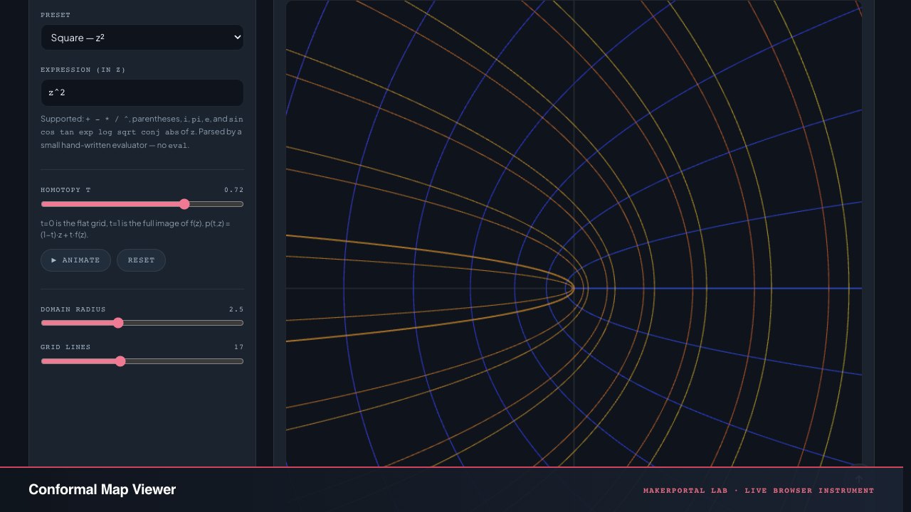
The instrument, captured—not illustrated.

This 16:9 frame is rendered from the real browser instrument above. It is the page's canonical preview for image search, link unfurls, and posts that need to show what the tool actually does.

Download 1280 × 720 JPEG

Conformal Mapping Explorer — live MakerPortal instrument screenshot — Canonical capture · real UI · no generated scientific artwork

Continue the experiment

All lab instruments →

Research

Conformal Map Viewer

f(z)