Playground · research instrument
DSP · AudioAcoustic Horn Calculator
Design acoustic horns and waveguides using the 1D Webster horn equation. Explore exponential, conical, and oblate spheroidal profiles and visualize their cross-sections in real time.
Independent research instrument — not claimed as MakerPortal shipped product code. Methods, equations, assumptions, and limitations are disclosed so you can inspect what the page does and does not establish.
Horn Parameters
Exit dimension
—
Mouth Dia. mm
Total exit area
—
Mouth Area cm²
Approx. low limit
—
Cutoff fc Hz
HF beamwidth
—
Directivity °
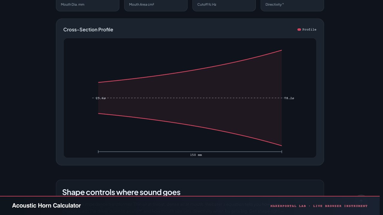
Cross-Section Profile
Shape controls where sound goes
A horn is an impedance transformer. Thin air at throat, dense air at mouth. Webster's equation tells you how area change loads the driver down to a cutoff, and how mouth size sets directivity when gets big. Get shape right — you keep directivity constant. Get it wrong — beam narrows, HOMs ring, response ripples.
1 — Webster: 1D horn physics
Assume pressure is uniform across cross-section, varies only along axis . Conservation of mass + momentum gives Webster:
is area profile. Solve for harmonic → spatial ODE whose solutions propagate only if above cutoff set by area flare rate. Ignore transverse modes — that is the core approximation. Valid up to depending on flare angle, beyond you need BEM.
2 — Three profiles, three bargains
Exponential: . Classic Keele / Klipsch. Area doubles every ln2/m. Loads driver with frequency-independent resistance above cutoff, then dies below:
Great LF loading, terrible directivity — beamwidth shrinks as because curved walls repeatedly reflect higher-order modes.
Conical: . Straight walls. Poor loading — no sharp , just gradual transformer — but wall angle sets beamwidth directly: full angle . That is constant directivity by geometry.
Oblate Spheroidal (OSWG): where governs throat curvature. Derived by Geddes: define oblate spheroidal coordinates so wavefronts are spherical caps. Matches flat piston to spherical expansion at mouth with minimal discontinuity, killing HOMs that plague exponential and rapid-flare horns. Best CD + low HOM, slight price in LF loading vs exponential.
3 — Directivity, ka, and why size matters
Mouth directivity kicks in when mouth circumference comparable to wavelength. Formal parameter:
$ka < 1$ → mouth omnidirectional, waveguide does little. → pattern control starts. $ka >5$ → strong beam. For constant directivity you want small enough that driver doesn't beam before waveguide takes over, and mouth large enough to hold pattern to lowest desired frequency: . That is why HF beaming shows as ___ in this canvas? The tool visual scales 1:1 so you can read mouth vs throat ratio immediately.
Beamwidth for rigid disk, but actual horn beam conical above .
4 — Playbook: choosing OSWG vs conical vs exponential
- Studio monitor CD: Use oblate spheroidal. Set throat to driver diameter (25.4 mm for 1"), length 150–250 mm, half-angle 40–50°. Mouth ends mm gives pattern control to ~1.2 kHz.
- PA long throw: Conical with 30° half-angle gives 60° nominal (−6 dB) beam that stays ~60° from 2 kHz to 16 kHz. Pay with LF loading — add separate mid horn below.
- Bass horn: Exponential wins. Choose from desired via . Example: Hz → . Then length sets mouth size: .
- HOM check: If flare changes slope abruptly (throat kink), you create higher-order modes that bounce and create time smear. OSWG curvature continuity fixes this — watch profile in canvas: smooth second derivative = good.
5 — Honesty: 1D is not 3D
Webster assumes planar or spherical isophase wavefronts. Real horn with wide angle, sharp walls, or diffraction slot launches transverse modes above . The tool does not predict those modes, nor diffraction at mouth edge, nor polar lobing, nor driver diaphragm breakup interacting with throat. Directivity number shown is geometric half-angle only, not measured DI. For accurate directivity maps () and throat impedance , run BEM (AKABAK, COMSOL, or open VACS). Use this designer to get first-cut area profile and mouth size that fits your cabinet, then validate with simulation and polar measurements.
Anatomy of the instrument
Three parameters, three profile types, one live cross-section canvas. Here is how the sliders connect to the Webster area function and how the canvas draws the horn walls at true 1:1 aspect ratio.
Parameters and the profile engine
- 01
Throat diameter → S₀. The first parameter sets the initial throat area . All three profile types use this as the starting area. For a 1" compression driver, the standard throat is 25.4 mm. The slider range (10–100 mm) covers everything from small tweeter throats to large-format midrange horns.
- 02
Flare parameter — dual identity. For exponential, this is the flare constant m (1/m), ranging 1–50. For conical and OSWG, it's the half-angle θ in degrees (5–85°), internally converted to radians. Switching profile type updates the label, slider range, and default value so the parameter never goes out of bounds.
- 03
Length → mouth size. The third parameter is total horn length L (10–500 mm). The
websterHornArea()function evaluates S(L) for the given profile: exponential gives , conical gives , OSWG gives where is derived from the half-angle. Mouth diameter is then . - 04
Cutoff and directivity outputs. For exponential, fc = m·c/(4π) — the frequency below which the horn doesn't load. For conical/OSWG, fc is not sharply defined (shown as "—"), and directivity is estimated as 2θ — the full geometric beamwidth. These are first-order approximations: real fc is influenced by mouth size, and real directivity depends on ka at the mouth.
The cross-section canvas
- 05
True 1:1 aspect ratio. The canvas enforces equal x and y scaling — the horn profile is not stretched. The scale is computed as where r_max is the mouth radius. This means very long/narrow horns fill the canvas width, and very wide horns are constrained by height. The result always shows the geometric shape accurately.
- 06
Area-to-radius conversion. The canvas samples 201 points along the horn axis, computing at each x via
websterHornArea(). Each S is converted to radius . The upper wall is drawn at , the lower wall at . The area between them is filled with semi-transparent magenta. - 07
Dimension annotations. Throat diameter is labeled at the left edge, mouth diameter at the right edge. A dimension line below the profile shows the total length in mm. The central axis is drawn as a dashed line. These labels update live as you drag sliders — compare different flare rates side-by-side by noting the mouth diameter at a fixed length.
- 08
Raf-throttled, no idle loop. Slider updates are batched via
requestAnimationFrame— changing any slider triggers a recompute of the mouth area, dashboard readouts, and canvas redraw in the next frame. There is no animation loop, no idle computation. The canvas also redraws on window resize and theme change via a MutationObserver ondata-theme.
The area functions defined
Exponential: . Conical: . OSWG: . All three share S₀ and converge at x=0. The difference is the second derivative: exponential accelerates, conical is constant d²S/dx², OSWG starts flat at the throat and smoothly transitions to spherical-cap expansion.
Gear for waveguide & horn measurement
Measurement stack · 18 picks
Audio interfaces & monitoring18
 $159.00Headphones
Audio-Technica ATH-M50X Professional Studio Monitor Headphones, Black, Professional Grade, Critically Acclaimed, with Detachable Cable
Reference monitoring headphones used for akous's binaural audio testing.
 $229.00Audio interface
Behringer UMC1820 Audiophile 18x20 USB Audio/MIDI Interface with Midas Mic Preamplifiers and ADAT I/O | For Recording Microphones and Instruments
Audio interface used building Biquadia — 8-preamp USB I/O for real-time DSP testing.
 $54.99Microphone
Blue Yeti Nano Premium USB Microphone - Shadow Grey (Renewed)
Compact USB condenser mic used for nymic testing.
 $9.99Audio
Comimark 1Pcs ADMP401 MEMS Microphone Breakout Module Board for Arduino Universal 1.3cm*1cm
MEMS mic breakout used for real-time DSP experiments feeding into Biquadia.
 $59.98Microphone
Dayton Audio EMM-6 Precision Omnidirectional Electret Condenser Microphone for Room Acoustic Analyzers and Audio Measurement Systems, Calibration Data File with Response Graph Included
Omni condenser with cal file — pair with REW to measure SPL, RT60, and comb filtering the acoustic calculator suite computes via image-source method.
 Microphone
Dayton Audio EMM-6 Precision Omnidirectional Electret Condenser Microphone for Room Acoustic Analyzers and Audio Measurement Systems, Calibration Data File with Response Graph Included
Latest EMM-6 variant with calibration file — measure waveguide polar response and cone-breakup waterfall to validate directivity index this lab computes.
 Microphone
Dayton Audio UMM-6 USB Measurement Microphone
USB cal mic for nearfield SPL and cone-breakup waterfall — capture the CSD breakup modes this simulator predicts via modal superposition.
 $39.98Tool
Focusound 24 Packs Acoustic Foam Panels Pyramid 2" X 12" X 12", Soundproofing Foam Noise Cancelling Foam with 120 PCS Double-Side adhesive
Pyramid foam taming room modes at f = n c / 2L — measure RT60 drop and compare to acoustic-calculator predictions for absorption coefficient vs frequency.
 Audio interface
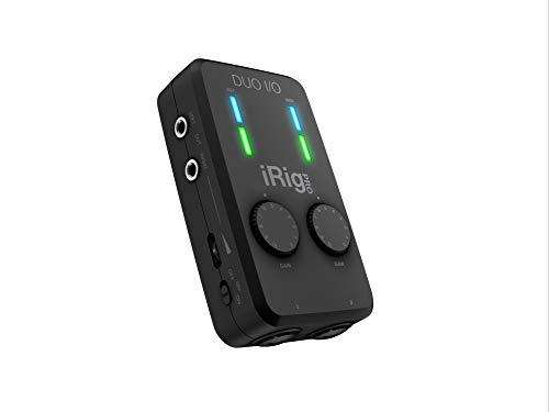
IK Multimedia iRig Pro Duo I/O USB audio interface, TRS balanced & headphones outputs, audio mixer to 24-bit, midi interface for music studio, recording, podcasting, streaming & social apps
Portable 2-channel USB-C audio interface used for mobile Biquadia field recording.
 $50.62Book
Loudspeaker Design Cookbook
Breakup modes, cone edge termination, and waveguide directivity index — chapters 7-9 explain the cone-breakup visualization and waveguide polar math this lab implements.
 $38.38Book
Master Handbook of Acoustics, Seventh Edition
Bible of RT60, Sabine, and absorption coefficients — the exact formulas these acoustic calculators implement for reverb, room modes, and critical distance.
 $168.00Microphone
RØDE NT-USB+ Professional-Grade USB Condenser Microphone for Recording
USB condenser mic used for nymic testing.
 $8.99Audio
SABRENT USB External Stereo Sound Card Adapter, Plug & Play (AU-MMSA)
USB audio interface used in early Biquadia MEMS-mic prototyping.
 Microphone
Sennheiser Pro Audio Sennheiser Pro Audio Wireless Microphone System, Black (MKE600)
Wireless mic system used for akous's ambient/binaural field recording.
 $319.00Microphone
Shure MV7+ USB-C & XLR Podcast Dynamic Mic with Stand - Black
USB/XLR hybrid mic used building and testing nymic.
 $237.00Microphone
Shure MV88+ USB-C Video Kit Stereo Condenser Microphone
Portable stereo condenser mic kit used for Biquadia field/video capture.
 $98.00Headphones
Sony MDR7506 Professional Large Diaphragm Headphone
Reference studio headphones used for akous's binaural audio testing.
 $98.91Book
The Physics of Musical Instruments
Modal analysis of plates and strings with Bessel functions — root of Chladni plate eigenmodes and waveguide modal cutoff fc = c/2a this toolbox computes.
Prices shown were retrieved from the Amazon Product Advertising API on 8 October 2026 and are indicative only — the price and availability on Amazon at the time of purchase apply.
More gear across every app: the full Gear list →
Two gotchas worth knowing
The 1D assumption breaks at wide angles
Webster's equation assumes isophase wavefronts are planar or spherical caps — pressure varies only along the axis, not across the cross-section. This holds for half-angles below ~30°. At 45° and above, transverse pressure variation becomes significant and higher-order modes (HOMs) appear. The tool will still compute an area profile and draw a cross-section, but the acoustic predictions (fc, directivity) become increasingly inaccurate. For wide-angle horns, use this for geometry only and verify acoustically with BEM.
The exponential flare rate m is wavelength-dependent in real horns
In a true exponential horn, m is constant. But many "exponential" horns in practice have a flare rate that changes along the length — the throat may expand slowly for loading, then the mouth flares more rapidly to reach the desired mouth size within a practical length. This tool uses strict mathematical exponentials with constant m. The cutoff frequency fc = m·c/(4π) only applies if the flare rate is truly constant over the entire length. Real horns with variable flare rates have a more gradual cutoff transition.
JavaScript — the horn profile solver
The websterHornArea() function that computes cross-sectional area at any point along the horn axis. Three profiles, one function, zero dependencies.
Horn area profile — JavaScript
const websterHornArea = (type, S0, param, x) => {
  if (x <= 0) return S0;
  switch (type) {
    case 'exponential': {
      return S0 * Math.exp(param * x);
    }
    case 'conical': {
      const r0 = Math.sqrt(S0 / Math.PI);
      return Math.PI * (r0 + x * Math.tan(param)) ** 2;
    }
    case 'oblate-spheroidal': {
      const r0 = Math.sqrt(S0 / Math.PI);
      const a = r0 / Math.tan(param);
      return S0 * (1 + (x / a) ** 2);
    }
    default:
      return S0;
  }
};

// Cutoff for exponential horns
const hornCutoff = (m, c = 343) => (m * c) / (4 * Math.PI);

// Mouth diameter from throat + profile + length
const mouthDiameter = (type, d0, param, L) => {
  const S0 = Math.PI * (d0 / 2) ** 2;
  const S_mouth = websterHornArea(type, S0, param, L);
  return 2 * Math.sqrt(S_mouth / Math.PI);
};
Frequently asked questions
What is the Webster horn equation and what does it assume?
Webster's equation is a 1D wave equation that assumes planar or spherical isophase wavefronts — pressure is constant across each cross-section and varies only along the horn axis. It's valid when the flare rate is moderate (wall angle < 30° half-angle) and ka < 3–5 at the throat. Beyond that, transverse (higher-order) modes appear and you need a 3D boundary element method (BEM) solver.
Which profile should I choose for a studio monitor waveguide?
Oblate spheroidal (OSWG). It transitions from a flat throat to a spherical-cap mouth with continuous second-derivative curvature, minimizing higher-order mode (HOM) generation at the throat-wall junction. Set throat to driver diameter (25.4 mm for 1"), length 150–250 mm, half-angle 40–50°. This gives pattern control below 1 kHz with a mouth diameter around 250–600 mm.
Why doesn't the conical horn have a defined cutoff frequency?
The conical horn's area grows as x² — it has no exponential flare rate m. There is no sharp cutoff like the exponential fc = m·c/(4π). Instead, loading drops gradually: the throat radiation impedance transitions from resistive at high frequencies to mass-like at low frequencies. Conical horns are used for constant-directivity applications (PA) where controlled beamwidth matters more than maximum loading efficiency.
How do I read the cross-section profile canvas?
The canvas shows a 1:1 true-aspect-ratio side view of the horn. The central dashed line is the axis. The upper and lower magenta curves are the horn walls — their gap at the left is the throat, and at the right is the mouth. The profile area is filled with a semi-transparent magenta tint. Throat diameter and mouth diameter are labeled at the ends. The total length is dimensioned below the profile. You can compare profiles side-by-side by switching types and watching the shape update.
What is the beamwidth number on the dashboard?
For conical and OSWG profiles, beamwidth is estimated as 2× the half-angle θ. A 45° half-angle gives ~90° nominal beamwidth. This is geometric directivity — it assumes ka at the mouth is large enough (>2–3) for pattern control to hold. At low frequencies where ka < 2, the mouth is acoustically small and beamwidth widens toward omnidirectional regardless of wall angle. The dashboard number is the high-frequency asymptote.
Shareable still
The instrument, captured—not illustrated.
This 16:9 frame is rendered from the real browser instrument above. It is the page's canonical preview for image search, link unfurls, and posts that need to show what the tool actually does.
Download 1280 × 720 JPEG