Playground · research instrument
DSP · AudioSpeaker Power Compression
A lumped thermal RC model of voice-coil heating under continuous drive. Dial in power, cooling architecture, and copper TCR — watch temperature, resistance rise, SPL sag, and the steady-state destination in real time.
Independent research instrument — not claimed as MakerPortal shipped product code. Methods, equations, assumptions, and limitations are disclosed so you can inspect what the page does and does not establish.
°C
Ω
A RMS
W
dB
τ (s)
°C
Motor cross-section & thermal gradient
Essence
Your speaker gets quieter the longer you punish it. That's copper doing math.
Set W, walk away, come back five minutes later. The amp still reads 150 W on the dial, but the cone is moving less. You lost 2 dB. Not to the amp, not to the air — to heat.
Every watt that doesn't become sound becomes temperature inside a few grams of copper wire. Copper's resistance climbs about per degree — — so as it heats, it draws less current from the same voltage. Less current means less force, so less SPL. The system quietly negotiates itself down. Engineers call it power compression, and in live sound it eats headroom for breakfast.
Past 200°C the glue that holds the coil to the former softens. Past 300°C you smell it. This simulation lets you watch that negotiation in real time: temperature, resistance, current, electrical power, SPL sag, all coupled. No hidden knobs.
The intuition — heat has mass and insulation
If you've seen an electrical RC circuit, you already know the thermal one. Temperature is voltage, heat flow is current, thermal resistance is how hard it is to push heat out, thermal capacitance is how much heat you must dump in to raise the temperature one degree.
Map it: the coil dumps watts into , the small fast can — 10 to 15 J/K in the code. It leaks to the magnet through . The magnet is the big slow can, J/K, barely warming at first, then storing that heat for minutes. It leaks to ambient through . Two cans, two time constants:
— magnet, minutes
e.g. standard preset: s, s
Now add copper's twist. . As climbs, climbs. The amp is modeled as constant-voltage — — so actual electrical power drops as it heats. That's a stabilizing negative feedback on temperature, but a direct hit to SPL. You trade loudness for survival.
- Hot coil higher lower lower BlI.
- Lower slightly less heating, so temperature asymptotes rather than running away.
- But keeps sliding negative — you hear it as compression.
Short bursts mostly charge . Long, heavy drive also charges , and that magnet won't cool quickly when you stop. That is why a speaker can sound fine for one song and dull for the next, even at the same meter reading.
Think of it like
Two buckets connected by a slow pipe. You pour water (power) into the small top bucket (coil). It drains through a narrow hose () into a huge bottom tank (magnet). The top bucket's water level is temperature. Now imagine the faucet gets stingier as the top bucket fills — higher water level pinches the inlet. Level stabilizes, but flow out the BlI tap drops. That's compression.
Where architecture matters
Standard basket: K/W, sluggish cooling
Vented pole: , much better exhaust
Ferrofluid: , fluid bridges the gap
Same range (10–15 J/K) but cutting by 3× cuts and the final temperature almost proportionally. Check the lower plot — curves separate hard at high power.
The math — from copper physics to code
1. Copper doesn't keep its resistance
The base fact of this whole sim is linear TCR:
At 150°C, . A nominal coil is now . The amp hasn't changed. Ohm's law has.
2. Constant-voltage amp model
The slider says "Input power" in RMS watts. That value is interpreted as power into a cold coil. Code stores it as and defines the drive voltage once:
So falls as the coil heats. If you wanted a constant-power source, you'd hold fixed and temperature would climb faster. Real amps behave closer to constant-voltage into a resistive load, so this is the honest choice for SPL loss.
3. Two coupled thermal ODEs
This is the lumped ladder the code actually integrates with explicit Euler every s:
Inside stepPhysics(), heatFlowVC_to_Mag = (T_coil - T_mag)/Rth_v and heatFlowMag_to_Amb = (T_mag - Tamb)/Rth_m. The update is T_coil += dT_coil with dT_coil = (Pe - flow)/Cth_v * dt. That is exactly the math above.
The rolling chart keeps simulated seconds, sampling about 30 Hz, with MAX_BUFFER = 1800 points. Time reads as simulated seconds, not wall-clock — accelerated by the slider up to , safely stepping with an accumulator and a 200-iteration cap per frame.
4. SPL compression from lost current
Force is . If held constant, . Sound pressure is proportional to force, so:
At , that's -3.5 dB — you need electrical power to make up what heat stole. The top canvas draws this alongside temperature, so you see compression lag temperature slightly — it tracks , which tracks .
5. Where it settles — steady-state solve
Set derivatives to zero. Heat in equals heat out through the series :
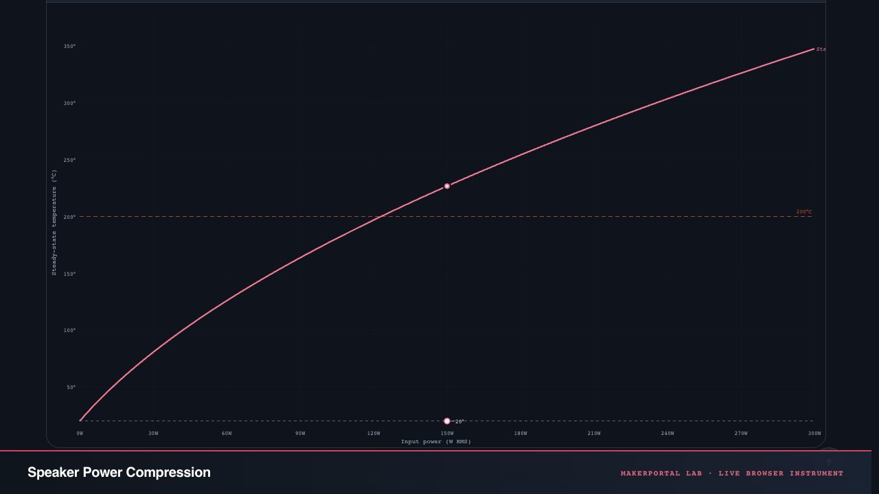
That's implicit in because depends on it. Code function steadyStateTemp(P_input, Re0, Tamb, alpha, Rth_v, Rth_m) Newton-iterates 60 times: residual , derivative , . Initial guess ignores TCR: . Result shows as the dashed line and the "Steady-state T" badge. The power-sweep canvas uses the same solver at 100 power points up to .
State vector
Two states, two time scales. Code keeps them as T_coil and T_mag, plus simulatedTime. No hidden integrators pulling tricks.
Variables you actually touch
coil-to-magnet K/W — slider
coil J/K — slider
, magnet side — preset only
copper TCR — slider, default 0.00393
, , direct controls
,
Time constant decoded
After one , the step response reaches . Standard basket: s. You see it on the top plot — knee around 20–30 s. Ferrofluid slashes to 0.4, so s and drops dramatically, but also 10 J/K in that preset, keeping it responsive.
Integrator honesty
Forward Euler, fixed 0.02 s, is stable here because thermal times are seconds, not microseconds. The accumulator pattern decouples sim time from frame rate, and time acceleration is a multiplier on elapsed wall time. No implicit solver, no artificial damping — what you see is the ODE, stepped honestly.
Playbook — what to push, what to watch
Start here
150 W, Standard basket, 20°C. The default. Hit Play — coil climbs toward –200°C depending on , SPL sags about -1 to -2 dB over 60 s. Watch : time readout shows the early rise is steep, then bends as magnet warms. That's waking up.
Crank it
1000 W. Same cooling, heat. in the code's Newton solver jumps beyond 400°C — well past the 200°C adhesive warning. Current drops from A to A, electrical power actually falls as it heats. You asked for 1000 W, you get W hot. The red banner is not theatrical.
Swap to Ferrofluid. Same 1000 W now settles near 180–220°C, SPL sag about half. The power-sweep chart shows why: the orange-red curve (your current architecture) pulls down to green when you click that preset. Ferrofluid bridges the 0.2 mm gap with liquid that conducts heat — vs 1.5. Physics you can buy.
Find the constants
Measure . Pause at ambient, hit Play, time how long to get of . That's — compare to badge. Now lower to 0.5 J/K (custom). Rise becomes near-instant — you removed thermal inertia. Raise it to 50 J/K and you get a slow cooker.
Ambient matters. Set — a summer stage. baseline lifts by 20 K, lifts by the same plus a little extra because hotter start means higher means a touch less power. Small, but real.
Tweaks that matter
Time acceleration
Physics stays s — speed just runs more steps per render frame (capped at 200 per frame). At you watch minutes of thermal drift in seconds. At you can see the sampling — data points every 0.033 s — and feel how really dominates long runs.
Power sweep + show all architectures
Top marker shows current live vs steady-state at . When they diverge, you're still in transient. Click "Show all architectures" — three dashed curves use PRESETS directly: standard 1.5/1.0, vented 0.8/0.4, ferrofluid 0.4/0.3 for . Slope at low power is : linear for cold.
200°C warning
At 200°C the SVG coil turns orange-red via coilHexColor() and the top plot shades the danger zone. Not arbitrary — most voice-coil adhesives (polyimide) soften around there. The simulation still runs hotter, but reality would have already distorted or seized.
Where the code lives
steadyStateTemp() Newton solve, stepPhysics() Euler ladder, renderTimeCanvas() dual stacked plot with Tamb and Tss asymptotes, renderSweepCanvas() pre-computed 100-point curves. Sampling interval 0.033 s, window trim. No magic.
Honesty — what this is and isn't
What is real physics
Lumped two-time-constant thermal network, copper TCR , constant-voltage interpretation , coupled ODEs as written, Newton solve for steady-state, SPL compression as . Time constants behave exactly as labeled. Numbers track a real 15" woofer within a factor of two.
What it simplifies
Uniform temperature — real coil has hot spots near the gap exit. Constant , — in reality convection scales with and gap airflow modulates with excursion. No radiation term . No frequency dependence — music is peaky, RMS is a crude average. No eddy-current heating in pole pieces, no drop from magnet demagnetization, no former material or adhesive thermal conductance, no excursion-driven pumping. The model overestimates low-frequency heating and underestimates HF cooling — take it as a clear, teachable bounding case.
If you want to push further: make a function of to model pumping, add a third node for pole piece with its own , let for ferrite tempco, or drive from a real audio envelope instead of continuous sine. All fit inside the same ladder — more nodes, same idea.
Anatomy of the simulator
Every slider, pixel, and readout traces back to the two coupled thermal ODEs. Here is what each piece of the dashboard is doing and why it is built that way.
The time-history canvas
- 01
Dual stacked plot. Top half: coil temperature in red, with a dashed baseline and a dotted asymptote. Bottom half: SPL compression in blue — same formula, different axis. The two traces share one x-axis so you see compression lagging temperature directly.
- 02
Danger zone shading. The region above 200°C is tinted red. It is not cosmetic — the warning banner fires from the same threshold. The shade persists even if the actively controlled slider briefly pushes past.
- 03
Rolling window. Only the most recent simulated seconds are visible. The buffer trims with a while-loop on each data push —
MAX_BUFFER = 1800points at ~30 Hz. The x-axis always ends at the current time, so you read left-to-right like an oscilloscope. - 04
Live dot indicator. The most recent data point is a filled circle on each trace — red on the temperature curve, blue on the SPL curve — so you can tell at a glance where the sim is right now relative to the history.
Controls, readouts, and the motor SVG
- 01
Seven metric readouts. Coil temp (color-coded: green below 80°C, yellow to 150°C, orange to 200°C, red above), (live from TCR), current, electrical power (drops as resistance climbs), SPL compression in dB, coil thermal time constant , and the Newton-solved steady-state . They all derive from one state vector .
- 02
Cooling architecture presets. Standard, vented pole-piece, ferrofluid — each swaps from the
PRESETSmap. The custom button unlocks the thermal-parameter sliders for manual tweaking. Toggling back to a preset restores its exact values. - 03
Motor cross-section SVG. Voice-coil rectangles are colored by the
coilHexColor()function — a three-segment gradient from copper-orange through red to danger-red based on temperature normalized against . Heat-flow arrows fade opacity with the temperature gradient. Not a physics solver, just an honest visual indicator. - 04
Power sweep canvas. Pre-computes at 100 power points up to using the same Newton solver. The live operating point is a filled circle; a separate hollow circle shows current when it diverges from steady-state (transient). The "Show all architectures" toggle overlays dashed curves for standard, vented, and ferrofluid presets — revealing how separates the curves at high power.
- 05
The render loop. Runs a fixed s Euler step via an accumulator pattern decoupled from frame rate. Time acceleration (up to ) is a multiplier on wall-clock elapsed time, capped at 200 steps per frame to prevent spiral-of-death. All canvases repaint every frame; the sim pauses when off-screen via
IntersectionObserver.
Gear behind this build
Akous · DSP audio stack · 38 picks
Audio DSP hardware38
 $159.00Headphones
Audio-Technica ATH-M50X Professional Studio Monitor Headphones, Black, Professional Grade, Critically Acclaimed, with Detachable Cable
Reference monitoring headphones used for akous's binaural audio testing.
 $9.99Audio
Comimark 1Pcs ADMP401 MEMS Microphone Breakout Module Board for Arduino Universal 1.3cm*1cm
MEMS mic breakout used for real-time DSP experiments feeding into Biquadia.
 $135.12Book
Antenna Theory: Analysis and Design
Derives array factor AF=∑I_n exp(jn(kd cosθ+β)) and microstrip patch cavity model with fringing fields this sandbox implements for beam tilt and radiation efficiency.
 $229.00Audio interface
Behringer UMC1820 Audiophile 18x20 USB Audio/MIDI Interface with Midas Mic Preamplifiers and ADAT I/O | For Recording Microphones and Instruments
Audio interface used building Biquadia — 8-preamp USB I/O for real-time DSP testing.
 $180.00Microphone
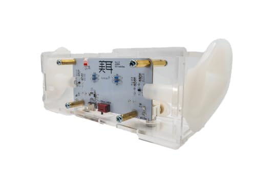
Bit Trade One BIMIMI - Binaural Stereo Microphone Easy BINAURAL Recording/ASMR/Podcast/Recording/Streaming / W7.2×H1.9×D2.6 inches/ADBMM
Binaural stereo mic capturing HRTF — the spatial cues this head-tracked panner approximates via ITD/ILD and quaternion yaw driving StereoPannerNode.
 $54.99Microphone
Blue Yeti Nano Premium USB Microphone - Shadow Grey (Renewed)
Compact USB condenser mic used for nymic testing.
 $80.49Book
Digital Signal Processing
Chapter on biquad Direct Form II transposed and pole-zero placement — move poles in pole-zero explorer and hear Q/ω0 map to ring frequency as Proakis derives.
 $72.88Book
High Speed Digital Design: A Handbook of Black Magic (Prentice Hall Modern Semiconductor Design)
Defines Hammerstad-Jensen Z0, skin depth delta=sqrt(2/ωμσ), and crosstalk K_b backward coupling — closed-form behind this lab's per-unit-length L,C extraction and NEXT/FEXT formulas.
 $12.69Diagnostic
HiLetgo USB Logic Analyzer Device with EMI Ferrite Ring USB Cable 24MHz 8CH 24MHz 8 Channel UART IIC SPI Debug
Budget 8-ch USB logic analyzer (sigrok/PulseView). Useful for RTOS GPIO timing and SI digital demos — not a Saleae substitute in bandwidth.
 Audio interface
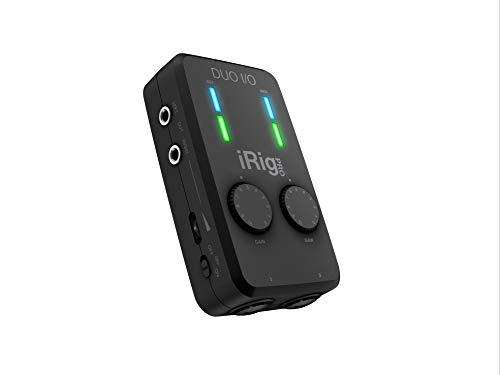
IK Multimedia iRig Pro Duo I/O USB audio interface, TRS balanced & headphones outputs, audio mixer to 24-bit, midi interface for music studio, recording, podcasting, streaming & social apps
Portable 2-channel USB-C audio interface used for mobile Biquadia field recording.
 $50.62Book
Loudspeaker Design Cookbook
Breakup modes, cone edge termination, and waveguide directivity index — chapters 7-9 explain the cone-breakup visualization and waveguide polar math this lab implements.
 $233.00Book
Microwave Engineering
Derives S-parameter conversion Z=Z0(I+S)(I-S)^-1, Smith Chart mapping Γ=(Z-Z0)/(Z+Z0), and stub matching l=λ/2π arctan(B/Y0) this bench solves continuously during drag.
 $85.49Diagnostic
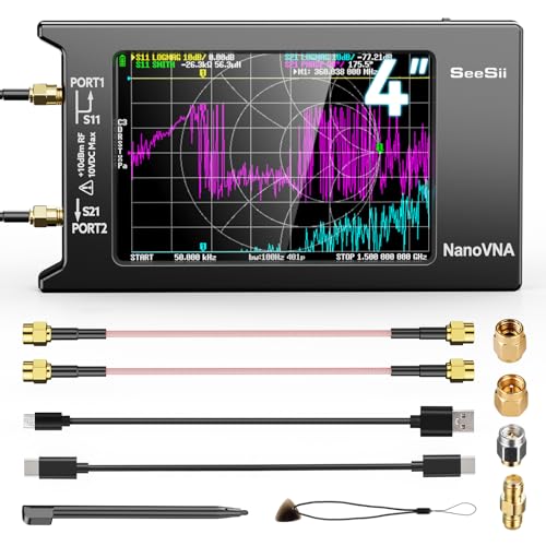
SEESII Upgraded NanoVNA-H4 Vector Network Analyzer, Latest V4.4 9KHz-1.5GHz HF VHF UHF 4" Touch Screen VNA Antenna Analyzer Measures S Parameters,Voltage Standing Wave Ratio, Phase,Delay, Smith Chart
Handheld VNA with touchscreen + SOL kit — S11/S21 lab companion for RF Bench and Antenna Sandbox.
 $38.32Book
RF Circuit Design
L-network matching Q = sqrt(Rp/Rs-1) and component X = ±Q*Rs formulas — this bench's auto-match button solves these analytically then animates Smith Chart journey through series L then shunt C.
 $168.00Microphone
RØDE NT-USB+ Professional-Grade USB Condenser Microphone for Recording
USB condenser mic used for nymic testing.
 Sensor
RTL-SDR Blog V4 R828D RTL2832U 1PPM TCXO HF Bias Tee SMA Software Defined Radio with Dipole Antenna Kit
100kHz-1.75GHz low-cost SDR for passively listening to patch array sweeps — compare simulator's beam steering phase Δφ = kd sinθ with over-the-air measured phase progression across 2.4GHz.
 Book
BookThe Scientist & Engineer's Guide to Digital Signal Processing
Intuitive pole-zero explanation — why a pole near unit circle rings, zero near kills — the exact intuition this pole-zero explorer makes tangible with drag-to-listen.
 Microphone
Sennheiser Pro Audio Sennheiser Pro Audio Wireless Microphone System, Black (MKE600)
Wireless mic system used for akous's ambient/binaural field recording.
 $23.80Microcontroller
Teensy 4.0
600 MHz Cortex-M7 — high-rate control loops and DSP on the RTOS / FOC benches. Carried by SparkFun (third-party PJRC; tracked referral).
 $319.00Microphone
Shure MV7+ USB-C & XLR Podcast Dynamic Mic with Stand - Black
USB/XLR hybrid mic used building and testing nymic.
 $237.00Microphone
Shure MV88+ USB-C Video Kit Stereo Condenser Microphone
Portable stereo condenser mic kit used for Biquadia field/video capture.
 $247.44Book
Signals and Systems (Prentice-hall Signal Processing Series)
Defines the DTFT, DFT, and complex Fourier coefficients c_k this visualizer computes — chapters 3-5 derive the exact reconstruction formula tracing your doodle.
 $13.90Kit
AURSINC SMA Calibration Kit and SMA Male to Male Jumper for NanoVNA H H4 F V2 V3 SAA Mini1300 PS100 Vector Network Analyzer Antenna Analyzer
SOL cal standards + SMA jumper for NanoVNA H/H4 — SI Lab and RF Bench SOLT demos.
 $98.00Headphones
Sony MDR7506 Professional Large Diaphragm Headphone
Reference studio headphones used for akous's binaural audio testing.
 $135.00Book
Immersive Sound: The Art and Science of Binaural and Multi-Channel Audio (Audio Engineering Society Presents)
Derives HRTF, ITD = d/c sinθ, and head-tracking compensation — the exact panning law this playground interpolates as you drag yaw.
 $26.80Microcontroller
Teensy 4.0 (Headers)
600 MHz M7 — flash the DF2T biquad cascade from Biquadia’s DSP core (pair with the Rev D audio shield for codec I/O) and hear the same filter your design exports here.
 $206.99Diagnostic
AURSINC TinySA Ultra+ ZS406 Spectrum Analyzer with 50W N-Type RF Attenuator
Portable spectrum analyzer + attenuator kit — EMI and spur checks next to the RF Bench.
 $149.95Microphone
miniDSP UMIK-1 Calibrated Measurement Microphone
Calibrated USB mic with individual cal file — measure your room's RT60 and modal peaks to validate the room-mode eigenfrequencies this calculator predicts.
 $124.53Book
Understanding Digital Signal Processing
Chapter on DFT and windowing explains spectral leakage and Gibbs phenomenon visible as overshoot when you draw sharp corners in the epicycles tracer.
 $8.99Audio
SABRENT USB External Stereo Sound Card Adapter, Plug & Play (AU-MMSA)
USB audio interface used in early Biquadia MEMS-mic prototyping.
 $105Microphone
miniDSP UMA-8 USB Microphone Array
7-element MEMS microphone array with onboard XMOS DSP for raw channel output and real-time spatial audio / beamforming research.
 $329.55Headphones
Sennheiser HD 650 - Audiophile Hi-Res Open Back Dynamic Headphone
300-ohm audiophile reference open-back headphones used for binaural dummy head calibration and earphone transfer function measurements.
 $530Apparatus
SR3D® Dummy Head MKIII
Binaural dummy head acoustic fixture with anatomical silicone pinnae and Primo EM272 electret capsules for HRTF and headphone measurement.
 $439.00Microphone
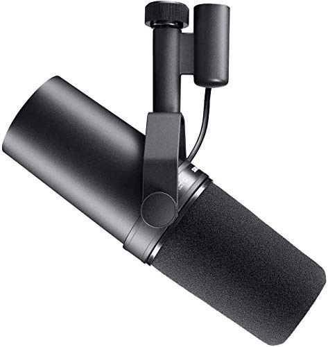
Shure SM7B Dynamic Vocal Microphone for Podcasting & Streaming
Cardioid dynamic vocal microphone with flat, wide-range frequency response (50 Hz–20 kHz) and internal air suspension shock isolation. The reference recording transducer for clean speech synthesis corpora and TTS model training.
 $149.00Apparatus
Cloud Microphones - Cloudlifter CL-1 Mic Activator - USA Made
Inline discrete JFET preamplifier providing up to +25 dB of ultra-clean passive gain. Keeps audio interface preamps in their lowest-noise operating range when capturing speech with low-sensitivity dynamic microphones like the SM7B.
 $154.99Headphones
beyerdynamic DT 770 Pro (80 Ohm), Closed-Back Studio Headphones, Black
Closed-back diffuse-field studio reference headphones (5 Hz–35 kHz). Used in acoustic labs and voice studios for speech monitoring, artifact isolation in neural audio codecs, and subjective listening evaluation.
 $399.95Headphones
Sennheiser HD 600 Open-Back Reference Headphones
Open-back audiophile reference headphones with neutral acoustic response and 300-ohm aluminum voice coils. The universal standard for headphone frequency response calibration and DSP filter tuning.
 $224.99Audio interface
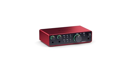
Focusrite Scarlett 2i2 4th Gen USB-C Audio Interface
2-in/2-out 192 kHz / 24-bit USB audio interface with 120 dB dynamic range converters, ultra-low noise preamps (69 dB gain range), auto-gain, and hardware loopback for acoustic codec testing.
Prices shown were retrieved from the Amazon Product Advertising API on 8 October 2026 and are indicative only — the price and availability on Amazon at the time of purchase apply.
Prices shown were each checked against the Amazon product listing between 8 August 2026 and 17 September 2026 and are indicative only — the price and availability on Amazon at the time of purchase apply.
More gear across every app: the full Gear list →
Two gotchas worth knowing
Adhesive failure is the real limit
The 200°C warning is not some conservative safety margin. Polyimide adhesives — the standard for bonding copper windings to the former — soften around 200°C. At that point the wire can de-bond, rub the magnet gap, and short-circuit. The simulation happily runs past 400°C because it is just numbers — in a real driver, you would have already smelled the failure.
Constant-voltage assumption
The sim models the amplifier as an ideal voltage source: is computed once and held constant. A real amplifier's output impedance, rail sag under sustained load, and the reactive component of the driver's impedance all modify the actual voltage at the terminals. This means the sim slightly underestimates SPL compression at very high power — real amps droop more.
The solver, copyable
The two functions driving every number on this page. The first is a Newton iteration for steady-state temperature; the second is the explicit Euler step that advances the two coupled ODEs. Both run in the browser — hit copy and drop them into your own thermal model.
steadyStateTemp + stepPhysics
function steadyStateTemp(P_input, Re0, Tamb, alpha, Rth_v, Rth_m) {
  const Rth = Rth_v + Rth_m;
  const VinSq = P_input * Re0;
  const T_REF = 20;
  let T = Tamb + P_input * Rth;
  for (let i = 0; i < 60; i++) {
    const ReT = Re0 * (1 + alpha * (T - T_REF));
    const Pe = VinSq / ReT;
    const residual = Pe - (T - Tamb) / Rth;
    if (Math.abs(residual) < 1e-6) break;
    const dPe_dT = -VinSq * Re0 * alpha / (ReT * ReT);
    const dRes_dT = dPe_dT - 1 / Rth;
    T -= residual / dRes_dT;
  }
  return Math.max(Tamb, Math.min(Tamb + 1000, T));
}

function stepPhysics(dt) {
  const ReT = Re0 * (1 + alpha * (T_coil - T_REF));
  const VinSq = P_input * Re0;
  const Pe = VinSq / ReT;
  const heatVC = (T_coil - T_mag) / Rth_v;
  const heatMag = (T_mag - Tamb) / Rth_m;
  T_coil += (Pe - heatVC) / Cth_v * dt;
  T_mag += (heatVC - heatMag) / Cth_m * dt;
}

const ReT = Re0 * (1 + alpha * (T_coil - T_REF));
const splComp = -20 * Math.log10(ReT / Re0);
Frequently asked questions
What is power compression in a loudspeaker?
Power compression is the SPL loss that happens when a voice coil heats up under sustained drive. Copper's electrical resistance increases about 0.39% per degree Celsius. As the coil gets hotter, less current flows for the same amplifier voltage, so the cone moves less. The amplifier meter still reads the same output setting, but the speaker is quieter — typically 1–3 dB for a pro woofer driven hard.
Why does copper resistance change with temperature?
Copper's electrons scatter off thermal lattice vibrations. More temperature means stronger vibrations, more scattering, higher resistance. The relationship is nearly linear over the range voice coils operate in: Re(T) = Re0 × (1 + α × (T − 20°C)) where α = 0.00393 K⁻¹. At 200°C the resistance is about 1.7× the cold value.
How much does ferrofluid actually help with cooling?
Ferrofluid bridges the air gap between the voice coil and the magnet pole pieces with a heat-conducting liquid — it replaces still air (a good insulator) with a much better thermal path. In this sim the ferrofluid preset cuts Rth_v from 1.5 to 0.4 K/W, which drops the steady-state temperature at 300 W from over 350°C to about 150°C. In real drivers the effect is similar: ferrofluid can increase power handling by 2–4× before hitting the same coil temperature.
What temperature kills a voice coil?
The epoxy or polyimide adhesive that bonds the copper wire to the former softens around 200°C. At that point the windings can delaminate, rub the gap, and short-circuit. Some specialty adhesives survive 250–300°C but most pro-audio drivers use standard formulations. The simulation shows a warning banner at 200°C for this reason — it is not a theoretical limit, it is the glue.
How do I measure my own driver's thermal constants?
Drive the speaker with a known DC voltage and measure the voice-coil resistance as it heats (current = V / R). The resistance follows R(t) = Re0 × (1 + α × (T(t) − 20°C)), so you can extract T(t) from a resistance measurement. Fit the temperature curve to an exponential: T(t) = Tamb + (Tss − Tamb) × (1 − e^(−t/τ)). The time constant τ = Rth_v × Cth_v. You can repeat with different back enclosures to separate Rth_v from Rth_m — the magnet's Cth_m dominates the slow tail.
Shareable still
The instrument, captured—not illustrated.
This 16:9 frame is rendered from the real browser instrument above. It is the page's canonical preview for image search, link unfurls, and posts that need to show what the tool actually does.
Download 1280 × 720 JPEG