Playground · research instrument
DSP · AudioPole-Zero Plot Tool
Drag poles and zeros on the z-plane. Watch the frequency response compute in real time from the exact transfer function H(z) — not an approximation. Preview the filter on live audio with Web Audio IIRFilterNode.
Independent research instrument — not claimed as MakerPortal shipped product code. Methods, equations, assumptions, and limitations are disclosed so you can inspect what the page does and does not establish.
Pole-zero filter explorer
z-Plane
Filter presets
Type: —
Pole position
r = 0.85, θ = 0.30 rad (— Hz at 48 kHz)
Zero position
r = 1.00, θ = 3.14 rad (— Hz at 48 kHz)
Biquad coefficients
b0 = 1.000000
b1 = -2.000000
b2 = 1.000000
a1 = -1.363538
a2 = 0.722500
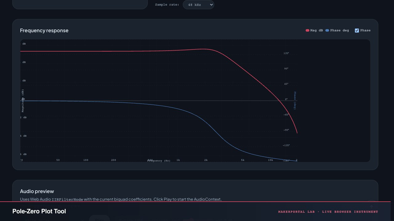
Frequency response
Audio preview
Uses Web Audio IIRFilterNode with the current biquad coefficients. Click Play to start the AudioContext, then toggle bypass to compare.
AudioContext not started — click Play
Anatomy of the explorer
Dragging a colored dot rewires the filter. Here is exactly what each piece of the UI does, under the hood.
The z-plane canvas
- 01
Cyan pole handles. Fill-drawn circles positioned at and — the conjugate pair. Dragging the top handle drags both: the bottom mirror tracks automatically, keeping coefficients real. The dashed line from origin to each pole shows radius visually — closer to the circle = sharper resonance.
- 02
Orange zero handles. Ring-drawn (outlined, not filled) to visually distinguish from poles. Same conjugate enforcement. Dashed connection lines anchor from origin. Zeros on the unit circle create perfect nulls — the edge of the zero handle is clipped to the circle, so you see exactly when a null is at the surface.
- 03
Unit circle with labels. The circle is the frequency axis: angle = frequency, counterclockwise from Re axis. Labels show Hz at current Fs at π/4 intervals. The radius grid maps the interior: center = 0 (no gain), edge = 1 (infinity for poles if stable clamp overridden).
What dragging actually computes
Every pointermove fires the full pipeline: polar → canvas coords → clamp r → derive biquad coefficients → evaluate H(e^jω) at 600 log-spaced frequencies → redraw both z-plane and response. This runs at 60 fps during drag with no perceptible lag because the math is just a few cos/sin calls per step.
Controls, render, and audio
- 01
Radius & angle sliders. Same data as dragging, but precise: the radius slider is a Q-knob in disguise ( near the circle), and the angle slider maps directly to frequency. Both show live readouts in Hz at the current sample rate.
- 04
Preset buttons. Six named filter types with exact r/θ values. Lowpass: zero at θ=π on circle, pole near θ=0. Bandpass: zero at origin r=0. Allpass: r_z = 1/r_p same angle. Each is a single biquad derived from pole-zero geometry — identical to the preset you would build in the Biquad Designer but visualized as positions instead of Q and f₀.
- 05
Web Audio chain. The IIRFilterNode is created with current feedforward [b0,b1,b2] and feedback [1,a1,a2] — the same six numbers. A ThemeObserver watches data-theme and redraws both canvases on change. A MutationObserver also teardowns the audio context on astro:before-swap.
Gear behind this build
DSP-audio stack · 16 picks
Audio hardware16
 Audio interface
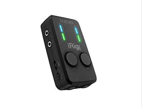
IK Multimedia iRig Pro Duo I/O USB audio interface, TRS balanced & headphones outputs, audio mixer to 24-bit, midi interface for music studio, recording, podcasting, streaming & social apps
Portable 2-channel USB-C audio interface used for mobile Biquadia field recording.
 $229.00Audio interface
Behringer UMC1820 Audiophile 18x20 USB Audio/MIDI Interface with Midas Mic Preamplifiers and ADAT I/O | For Recording Microphones and Instruments
Audio interface used building Biquadia — 8-preamp USB I/O for real-time DSP testing.
 $9.99Audio
Comimark 1Pcs ADMP401 MEMS Microphone Breakout Module Board for Arduino Universal 1.3cm*1cm
MEMS mic breakout used for real-time DSP experiments feeding into Biquadia.
 $159.00Headphones
Audio-Technica ATH-M50X Professional Studio Monitor Headphones, Black, Professional Grade, Critically Acclaimed, with Detachable Cable
Reference monitoring headphones used for akous's binaural audio testing.
 $54.99Microphone
Blue Yeti Nano Premium USB Microphone - Shadow Grey (Renewed)
Compact USB condenser mic used for nymic testing.
 $110.61Book
DAFX: Digital Audio Effects
Biquad-based effects: peaking, shelving, allpass for phaser — agentic pipeline's RAG over DAFX generates the same C++ kernel clang++ verifies here.
 $80.49Book
Digital Signal Processing
Chapter on biquad Direct Form II transposed and pole-zero placement — move poles in pole-zero explorer and hear Q/ω0 map to ring frequency as Proakis derives.
 $168.00Microphone
RØDE NT-USB+ Professional-Grade USB Condenser Microphone for Recording
USB condenser mic used for nymic testing.
 Book
BookThe Scientist & Engineer's Guide to Digital Signal Processing
Intuitive pole-zero explanation — why a pole near unit circle rings, zero near kills — the exact intuition this pole-zero explorer makes tangible with drag-to-listen.
 Microphone
Sennheiser Pro Audio Sennheiser Pro Audio Wireless Microphone System, Black (MKE600)
Wireless mic system used for akous's ambient/binaural field recording.
 $319.00Microphone
Shure MV7+ USB-C & XLR Podcast Dynamic Mic with Stand - Black
USB/XLR hybrid mic used building and testing nymic.
 $237.00Microphone
Shure MV88+ USB-C Video Kit Stereo Condenser Microphone
Portable stereo condenser mic kit used for Biquadia field/video capture.
 $247.44Book
Signals and Systems (Prentice-hall Signal Processing Series)
Defines the DTFT, DFT, and complex Fourier coefficients c_k this visualizer computes — chapters 3-5 derive the exact reconstruction formula tracing your doodle.
 $98.00Headphones
Sony MDR7506 Professional Large Diaphragm Headphone
Reference studio headphones used for akous's binaural audio testing.
 $124.53Book
Understanding Digital Signal Processing
Chapter on DFT and windowing explains spectral leakage and Gibbs phenomenon visible as overshoot when you draw sharp corners in the epicycles tracer.
 $8.99Audio
SABRENT USB External Stereo Sound Card Adapter, Plug & Play (AU-MMSA)
USB audio interface used in early Biquadia MEMS-mic prototyping.
Prices shown were retrieved from the Amazon Product Advertising API on 8 October 2026 and are indicative only — the price and availability on Amazon at the time of purchase apply.
More gear across every app: the full Gear list →
The math and physics, in full
Every filter boils down to poles and zeros in the complex plane. Here is how they interact geometrically to shape the frequency response of the system.
How it works — poles push, zeros pull
1. Why the z-plane is the real story
Magnitude plots lie by omission. They show what a filter does, not why. The z-plane shows why. Every filter is just places where it blows up (poles) and places where it nulls (zeros). Move a dot, the whole frequency response reshapes because distance from that dot to the unit circle is gain. This playground makes that geometry tactile — drag a pole, hear resonance rise — instead of hiding it behind f0 and knobs. For the knob view, see Biquad Filter Designer.
2. Intuition — angles are frequency, radius is damping
Imagine the unit circle is a clock that runs 0 to Fs/2. Angle around that circle is frequency: . Radius is how sharp the resonance is. A pole at near boosts around Fs * 0.125 Hz. Drag it to and it rings like a cowbell. Drag it outside and the filter explodes — infinite amplitude, unstable.
3. The math — from geometry to biquad coeffs
One conjugate pole pair at and one zero pair at is a biquad:
4. How to play
Drag first: Grab the cyan pole, drag outward — resonance sharpens, magnitude peak rises from 3 dB to 30 dB.
5. Honesty check
This is a single biquad. Real equalizers cascade 4–12 — see Biquad Designer for that.
Two gotchas worth knowing
Stability clamp hides real math
Poles outside the unit circle are a real thing — they model unstable systems and intentionally growing oscillations. But in an audio filter, |p| ≥ 1 means infinite amplitude and a blown IIRFilterNode. We clamp to 0.995 max. If you remove the clamp in the code, drag a pole past the circle and listen to white noise become silence — the browser kills the filter to protect your speakers.
Conjugate enforcement limits topology
We always create two poles and two zeros as conjugate pairs. That forces real coefficients (your DSP needs them). But it also means you cannot place a single real pole on the Re axis — a first-order lowpass (one real pole at z = 0.9) is off-limits. The biquad is second-order always. For order-1 filters (DC blocker, simple leaky integrator), you would use directly, not this tool.
Copyable solver: pole-zero → biquad → response
These functions drop directly into any JS/TS DSP project. Feed them r, θ for one pole pair and one zero pair, get back normalized biquad coefficients and the frequency response vector.
TypeScript — dsp.ts (poleZeroToCoeffs)
// poles: [{r, theta}], zeros: [{r, theta}] — conjugate pairs
export function poleZeroToCoeffs(
  poles: {r:number, theta:number}[],
  zeros: {r:number, theta:number}[]
): {b0:number,b1:number,b2:number,a1:number,a2:number} {
  // numerator from zeros: (1 - z1 z^-1)(1 - z2 z^-1)
  const zr = zeros[0].r, zt = zeros[0].theta;
  const b0 = 1;
  const b1 = -2 * zr * Math.cos(zt);
  const b2 = zr * zr;
  // denominator from poles: (1 - p1 z^-1)(1 - p2 z^-1)
  const pr = poles[0].r, pt = poles[0].theta;
  const a1 = -2 * pr * Math.cos(pt);
  const a2 = pr * pr;
  return { b0, b1, b2, a1, a2 }; // a0=1, already normalized
}
TypeScript — freqResponse
export function freqResponse(
  coeffs: {b0:number,b1:number,b2:number,a1:number,a2:number},
  f: number, Fs: number
): {mag:number, phase:number} {
  const w = 2*Math.PI*f/Fs;
  const cosw = Math.cos(w), sinw = Math.sin(w);
  const cos2w = Math.cos(2*w), sin2w = Math.sin(2*w);
  // numerator: b0 + b1 e^-jw + b2 e^-j2w
  const nr = coeffs.b0 + coeffs.b1*cosw + coeffs.b2*cos2w;
  const ni = -coeffs.b1*sinw - coeffs.b2*sin2w;
  // denominator: 1 + a1 e^-jw + a2 e^-j2w
  const dr = 1 + coeffs.a1*cosw + coeffs.a2*cos2w;
  const di = -coeffs.a1*sinw - coeffs.a2*sin2w;
  const denom = dr*dr + di*di || 1e-12;
  const re = (nr*dr + ni*di) / denom;
  const im = (ni*dr - nr*di) / denom;
  return { mag: Math.hypot(re,im), phase: Math.atan2(im,re) };
}
Frequently asked questions
Why are poles and zeros always in conjugate pairs?
Real-valued time-domain signals need real-valued coefficients. A complex pole or zero on its own would produce complex coefficients (b0-b2, a1-a2). Pairing it with its complex conjugate makes the imaginary parts cancel out, keeping all coefficients real. The conjugate pair is mathematically equivalent to 2 cos θ and r² terms in the biquad denominator and numerator, which is why a single biquad always has one pair of poles and one pair of zeros.
What happens when a pole is exactly on the unit circle?
A pole on |z| = 1 means the denominator hits zero at that frequency — the response goes to infinity. In a real IIR filter, this produces an oscillator: a sine wave that sustains forever without decay. It is marginally stable (BIBO fails if you hit that exact frequency) but useful for tone generators. Digital waveguide synthesis uses poles on the unit circle to model undamped piano strings and flute bores.
How does the z-plane relate to analog s-plane design?
Analog filters are designed in the s-domain (Laplace) where the jω axis is the frequency axis and poles must lie in the left half-plane for stability. The bilinear transform maps s = (2/T)(1 − z⁻¹)/(1 + z⁻¹), warping the entire left half-plane into the unit circle. This is why RBJ cookbook formulas exist: they pre-warp ω₀ before analog prototype design so that the digital f₀ lands exactly where you want it after bilinear transformation.
Can I hear the difference between a lowpass and a notch?
Yes — very clearly. A lowpass at 1 kHz with Q = 0.707 removes everything above the cutoff smoothly, like turning down a treble knob. A notch with the same f₀ and a tight Q carves out a narrow band — a sine sweep through a sharp notch sounds like a hole punched in the frequency spectrum. Click the presets, toggle between them, and play white noise to hear the difference. The z-plane shows why: the notch puts a zero on the circle exactly at that angle.
Why is group delay not shown on this plot?
Group delay is the negative derivative of phase with respect to frequency: gd = −d(arg H)/dω. It tells you how many samples of delay each frequency experiences. We plot phase directly, and the slope you see is the group delay. Computing the exact derivative requires finite differences or analytic formulas — we have it in the codebase (dsp.ts) but chose to keep the plot focused on the two primary views (mag + phase) that change most visually as you drag.
Shareable still
The instrument, captured—not illustrated.
This 16:9 frame is rendered from the real browser instrument above. It is the page's canonical preview for image search, link unfurls, and posts that need to show what the tool actually does.
Download 1280 × 720 JPEG