Playground · research instrument
DSP · AudioDriver Nonlinearity Lab
A lumped-parameter moving-coil loudspeaker model with nonlinear Bl(x), Kms(x), and Le(x). Explore how force-factor droop and suspension stiffening generate harmonic distortion as excursion grows — educational, not measurement-grade.
Independent research instrument — not claimed as MakerPortal shipped product code. Methods, equations, assumptions, and limitations are disclosed so you can inspect what the page does and does not establish.
Drive & Parameters
Adjust drive level and nonlinearity coefficients.
- Peak excursion
- —
- THD estimate
- —
- Bl(x) at peak
- —
- Kms at peak
- —
The motor is linear until you ask it to work
Thiele-Small looks innocent at 1 watt. Push a driver to and three curves betray you: falls when coil leaves the gap, stiffens when spider and surround stretch, breathes with position. Each one is a distortion generator. This lab lets you dial them and watch the sine turn into something else.
1 — Bl(x): force factor droop
Ideal motor gives constant . Real gap has finite height. As coil moves out, fewer turns sit in -field. Force per amp drops. If coil is centered, droop is symmetric; if offset (common after sag or assembly), one side drops earlier — even-order distortion.
is asymmetry/shape knob. In Klippel measurements you see a bell curve, not this triangle — peak at rest, down to 70% at for a good long-throw, 50% for a cheap one. Twice excursion → twice loss → current has to rise → more heat → more compression. That coupling is outside this model, but you feel it in the motor SVG when status flips to "Coil out of gap".
2 — Kms(x): spider gets angry
Suspension compliance is progressive. Small , soft. Large , spider fibers align, surround folds stretch — stiffness climbs quadratically. This is symmetric by nature, so it makes odd harmonics.
Fixed Hz here gives . multiplies the square term. is a soft progressive spider, is a harsh bottoming surround. Because force is , you get an term — same math that makes a Duffing oscillator generate 3rd harmonic. Push Vrms and watch waveform flatten on peaks.
3 — Le(x): inductance modulates
Voice-coil inductance depends on how much steel it overlaps. Move out, drops ~. That sounds harmless until you realize impedance changes with position, so current waveform distorts even with perfect voltage drive. Add flux modulation (current itself modulates ) and you get — not modeled here but measured by Klippel .
The back-EMF is velocity times force factor — it fights input voltage. When droops at peak , back-EMF collapses, current spikes. That spike hits non-flat and you have intermodulation. In the canvas lower half, watch bell shrink with and dot trace current position.
4 — Where distortion comes from: Taylor tells all
Any memoryless nonlinearity can be expanded:
Drive :
So asymmetric → even order (2nd), symmetric → odd order (3rd). Real driver does both. THD here computed from displacement spectrum via numerical harmonic extraction:
Klippel's measurement rig does this for real with laser and current sense, plotting , , versus . Golden rule: keep above 80% and within 50% over intended . Once outside, no motor feedback fixes mechanical bottoming.
5 — Playbook & honesty
How to use
- Set V, Hz, , — this is a decent 6" woofer. Waveform looks sinusoidal, THD 2–5%, dot stays near top.
- Now push Vrms to 30 V or drop to 2 mm. Excursion exceeds gap, coil dot leaves bell, displacement waveform flattens, 3rd harmonic bar pops up in spectrum.
- Isolate mechanisms: , → pure suspension odd distortion. , → even. Combine — you get real driver stew.
- Lower raises acceleration , raises via — lighter cone distorts more at high freq? Check.
What this omits
Euler at 8 kHz timestep, no flux modulation , no eddy-current hysteresis in pole, no thermal memory, no cone breakup, no port nonlinearity, no equivalent circuit of , . , , shapes are simplified polynomials — real curves have asymmetry, plateau, and hysteresis loops. THD is displacement THD via 1024-sample history, not acoustic SPL THD. Use for qualitative cause → effect, not for validating a driver design. For that, need Klippel LSI or laser vibrometer.
Anatomy of the instrument
A real-time ODE solver at 8 kHz, two live canvases, an animated motor SVG, and a harmonic analyzer. Here is what each piece computes and how the render loop ties them together.
The physics engine and motor SVG
- 01
Euler integration at 8 kHz. Three state variables — displacement x, velocity v, current i — updated via forward Euler with s. Each step: compute , , from the current x, then integrate: , , , . A 1024-sample circular buffer stores displacement and voltage history for waveform display and harmonic extraction.
- 02
Run/pause with fixed timestep accumulation. The
renderFrame()callback measures elapsed wall-clock time and accumulates physics steps. When running, up to 5000 steps are processed per frame to prevent spiral-of-death if the tab loses focus. The accumulator caps at 0.05 s per frame to prevent bursts. When paused, physics freezes but canvases still redraw — you can study a frozen state. - 03
Animated motor SVG. The coil-group, cone, and force arrow translate vertically based on the historical peak excursion scaled to ±30 px. The gap indicator dims when |x| exceeds Xmax, and the status label switches from "Coil in gap" to "Coil out of gap" styled in the theme's magenta color. The force arrow length scales with — you see the motor push weaken as the coil leaves the gap.
- 04
THD from harmonic extraction. Every frame, the
extractHarmonics()function from the DSP library performs numerical Fourier integration over the 1024-sample displacement buffer at the drive frequency and its first three harmonics. THD = √(H₂²+H₃²+H₄²)/H₁ × 100%. This is computed synchronously in the animation loop — no FFT, no windowing overhead.
The two canvases
- 05
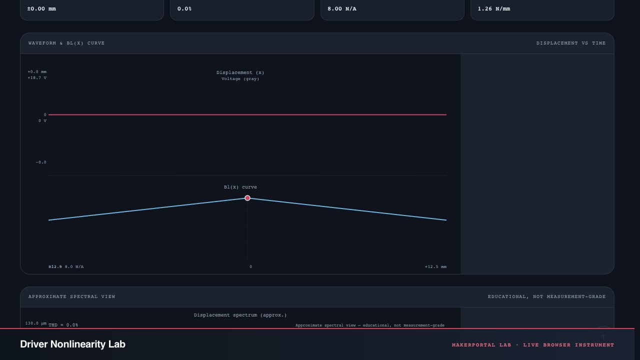
Waveform canvas (top). Upper half: displacement (magenta, 2 px) and input voltage (gray, 1 px) over the full 1024-sample history window. Auto-scaled symmetrically so the zero line stays at the midpoint. The y-axis labels show the current voltage and displacement ranges. Lower half: the curve — a tent shape whose width is set by Xmax and whose height is . A magenta dot marks the current operating point on the curve.
- 06
Spectrum canvas (bottom). Up to four harmonic bars positioned by their frequency on a linear x-axis from 0 to 5×f₀. The fundamental (f₀) bar uses the magenta color; harmonics 2–4 use blue. Each bar is labeled with its harmonic order and displacement amplitude in mm. The THD readout in the top-left corner matches the metric card. The maximum amplitude is auto-scaled to 1.3× the largest harmonic.
- 07
Visibility-aware frame skipping. An IntersectionObserver watches the motor card. When the page is scrolled off-screen or the tab is hidden, the render loop skips canvas drawing (but continues physics accumulation). This prevents wasting GPU on invisible canvases while maintaining physics continuity for when the user scrolls back.
- 08
Respects reduced-motion. On page load, the script checks
prefers-reduced-motion. If the user has that preference enabled, the simulation starts paused so no animation runs automatically.
The rendering loop
Each frame: if running, accumulate elapsed time into physics steps. Then call syncControls() (update metrics, animate SVG) and renderPlots() (redraw both canvases from the circular buffer). The canvases use setupHiDPI() for retina-quality rendering. On theme change, all canvases redraw automatically via a MutationObserver.
Gear for driver measurement
Measurement stack · 14 picks
Audio interfaces & monitoring14
 $159.00Headphones
Audio-Technica ATH-M50X Professional Studio Monitor Headphones, Black, Professional Grade, Critically Acclaimed, with Detachable Cable
Reference monitoring headphones used for akous's binaural audio testing.
 $229.00Audio interface
Behringer UMC1820 Audiophile 18x20 USB Audio/MIDI Interface with Midas Mic Preamplifiers and ADAT I/O | For Recording Microphones and Instruments
Audio interface used building Biquadia — 8-preamp USB I/O for real-time DSP testing.
 $54.99Microphone
Blue Yeti Nano Premium USB Microphone - Shadow Grey (Renewed)
Compact USB condenser mic used for nymic testing.
 $9.99Audio
Comimark 1Pcs ADMP401 MEMS Microphone Breakout Module Board for Arduino Universal 1.3cm*1cm
MEMS mic breakout used for real-time DSP experiments feeding into Biquadia.
 Audio interface
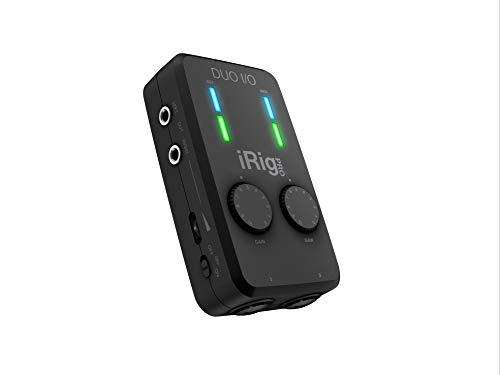
IK Multimedia iRig Pro Duo I/O USB audio interface, TRS balanced & headphones outputs, audio mixer to 24-bit, midi interface for music studio, recording, podcasting, streaming & social apps
Portable 2-channel USB-C audio interface used for mobile Biquadia field recording.
 $38.99Tool
JuviPerpric Digital K Type Thermocouple Thermometer, Dual Channel Thermocouple Tester(-238~3212℉) with 2 Temperature Clamp and 2 Wired Thermocouple Probes
Probe voice-coil former temperature and log T_vc(t) — compare measured τ_thermal rise against this lab's first-order thermal RC model with ferrofluid cooling.
 $50.62Book
Loudspeaker Design Cookbook
Breakup modes, cone edge termination, and waveguide directivity index — chapters 7-9 explain the cone-breakup visualization and waveguide polar math this lab implements.
 $168.00Microphone
RØDE NT-USB+ Professional-Grade USB Condenser Microphone for Recording
USB condenser mic used for nymic testing.
 $8.99Audio
SABRENT USB External Stereo Sound Card Adapter, Plug & Play (AU-MMSA)
USB audio interface used in early Biquadia MEMS-mic prototyping.
 Microphone
Sennheiser Pro Audio Sennheiser Pro Audio Wireless Microphone System, Black (MKE600)
Wireless mic system used for akous's ambient/binaural field recording.
 $319.00Microphone
Shure MV7+ USB-C & XLR Podcast Dynamic Mic with Stand - Black
USB/XLR hybrid mic used building and testing nymic.
 $237.00Microphone
Shure MV88+ USB-C Video Kit Stereo Condenser Microphone
Portable stereo condenser mic kit used for Biquadia field/video capture.
 $98.00Headphones
Sony MDR7506 Professional Large Diaphragm Headphone
Reference studio headphones used for akous's binaural audio testing.
 $24.95Book
Testing Loudspeakers
Step-by-step measurement of Thiele-Small, K_ms(x), Le(x) — same nonlinearities the loudspeaker nonlinearity lab models with displacement-dependent Bl(x) and stiffness.
Prices shown were retrieved from the Amazon Product Advertising API on 8 October 2026 and are indicative only — the price and availability on Amazon at the time of purchase apply.
More gear across every app: the full Gear list →
Two gotchas worth knowing
Forward Euler is conditionally stable at 8 kHz
The solver uses explicit Euler integration — the simplest possible numerical method. At 8 kHz timestep, the mechanical resonance (40 Hz) is well-resolved (~200 samples per cycle) and the electrical time constant Le/Re ≈ 0.08 ms is just barely stable. If you set extreme parameter combinations (very low Re + very high Le via large δ), the current integration can go unstable and blow up. The tool caps Le at reasonable values to prevent this, but it's a reminder that this is an educational model, not a production circuit simulator.
THD from displacement is not THD from SPL
The THD metric analyzes the displacement waveform — how much the cone motion deviates from a pure sine. Acoustic THD depends on additional factors: the cone's radiation impedance, breakup modes that filter displacement into SPL differently at each frequency, air nonlinearity at high SPL, and port distortion in vented boxes. Displacement THD is typically 2–5× lower than measured acoustic THD at bass frequencies and can be higher or lower at mid frequencies depending on breakup. Treat the THD number here as a lower bound on total harmonic distortion.
JavaScript — the nonlinear ODE solver
The core time-stepping loop. Three state variables, three nonlinear curves, one Euler integrator. This is the engine behind the animated SVG and waveform canvases.
Nonlinear driver step — JavaScript
const stepPhysics = (state, dt, t) => {
  const omega = 2 * Math.PI * state.freq;
  const vin = state.vrms * Math.sqrt(2) * Math.sin(omega * t);

  // Nonlinear force factor: drops as coil leaves gap
  const bl = state.bl0 * (1 - state.beta
    * Math.abs(state.x / (state.xmax || 1e-9)));

  // Suspension stiffness: progressive quadratic stiffening
  const kms0 = state.mms * (2 * Math.PI * 40) ** 2;
  const kms = kms0 * (1 + state.gamma
    * (state.x / (state.xmax || 1e-9)) ** 2);

  // Inductance modulation with position
  const le0 = 0.5e-3;
  const le = le0 * (1 + state.delta
    * Math.abs(state.x / (state.xmax || 1e-9)));

  // State update: forward Euler
  const di = (vin - state.re * state.i - bl * state.v) / le * dt;
  state.i += di;
  const a = (bl * state.i - kms * state.x) / state.mms;
  state.v += a * dt;
  state.x += state.v * dt;

  return { x: state.x, v: state.v, i: state.i, bl, kms, le };
};
Frequently asked questions
What exactly do β, γ, and δ control?
β (0–1) controls Bl(x) asymmetry — how much the force factor drops as the coil leaves the magnetic gap. γ (0–1) controls Kms(x) progressive stiffening — spider and surround getting stiffer with excursion. δ (0–1) controls Le(x) modulation — how voice coil inductance changes with position. Set each to 0 to isolate the others; real drivers exhibit all three simultaneously. Typical values for a mid-range 6" woofer: β≈0.1, γ≈0.2, δ≈0.05.
Why does the displacement waveform flatten at high drive?
That's Kms(x) stiffening. As excursion grows, the suspension spring constant increases quadratically (Kms ∝ 1 + γ·(x/Xmax)²), so the restoring force grows faster than displacement. The waveform clips symmetrically — both positive and negative peaks compress. This is a Duffing oscillator and it generates odd harmonics (3rd, 5th). Increase γ to 0.8 and watch the waveform square off.
Is the THD number accurate to real measurements?
No. This THD is computed from the displacement waveform using numerical harmonic extraction over a 1024-sample window — it's displacement THD, not acoustic SPL THD. Acoustic THD includes additional sources: cone breakup, port nonlinearity, air nonlinearity at high SPL, and microphone distortion. The tool is educational: it shows which nonlinearity produces which harmonic pattern. For real driver validation you need a Klippel LSI or laser vibrometer.
What happens when the coil leaves the gap?
The motor SVG shows the coil position relative to the magnet gap. When "Coil out of gap" appears, Bl(x) has dropped significantly — the force per amp is reduced. Current spikes because back-EMF (Bl·v) collapses, and the remaining force is applied through a stiffer suspension. The result is intermodulation distortion: the current waveform interacts with the position-dependent force factor to produce sum and difference frequencies. This is why drivers sound harsh when overdriven.
Why does changing Mms affect fs and distortion?
The tool ties Kms₀ to Mms via the fixed fs = 40 Hz: Kms₀ = Mms·(2π·40)². Heavier cone means higher Kms₀ to maintain the same resonance frequency. But the nonlinear Kms(x) model then applies γ to this higher baseline, so a heavier driver with the same γ is actually stiffer at any given excursion. This is realistic — adding mass without redesigning the suspension increases effective compliance nonlinearity.
Shareable still
The instrument, captured—not illustrated.
This 16:9 frame is rendered from the real browser instrument above. It is the page's canonical preview for image search, link unfurls, and posts that need to show what the tool actually does.
Download 1280 × 720 JPEG