Playground · research instrument
DSP · AudioSpeaker Cone Breakup Simulator
An illustrative modal-shape explorer — not an FEA simulation. Explore how a circular membrane/plate transitions from rigid-piston motion to modal breakup as frequency increases. Tune material, cone diameter, and frequency to see radial modes, nodal circles, and the qualitative frequency response.
Independent research instrument — not claimed as MakerPortal shipped product code. Methods, equations, assumptions, and limitations are disclosed so you can inspect what the page does and does not establish.
This is an illustrative modal-shape explorer, not an FEA simulation. A loudspeaker cone behaves as a rigid piston at low frequencies — every point on the surface moves in phase. As frequency rises past the first breakup mode, radial modes appear (concentric rings moving out of phase). At higher frequencies, complex modal patterns emerge with multiple nodal circles and diametral lines. The breakup frequency depends on material stiffness, density, and cone geometry:fbreakup ∝ √(E/ρ) / D, where E is Young's modulus, ρ is density, and D is the cone diameter.
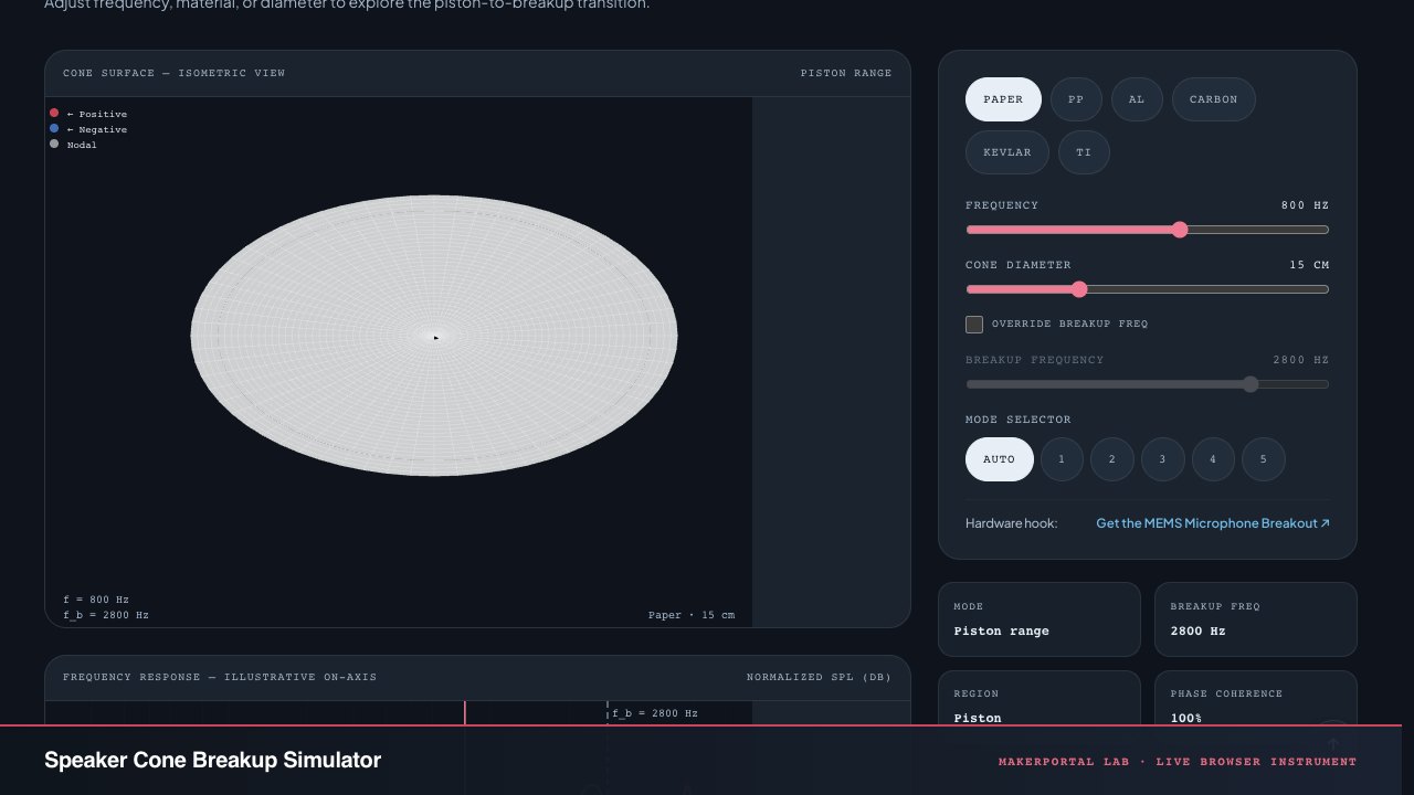
Cone breakup visualized
Adjust frequency, material, or diameter to explore the piston-to-breakup transition.
Mode shape selector
Mode selector
- Mode
- Piston range
- Breakup freq
- 2,800 Hz
- Region
- Piston
- Phase coherence
- 100%
How a cone stops being a piston
At low frequency your cone is a perfect piston. At high frequency it forgets. Bending waves race across it, hit the edge, reflect, and stand still. That is breakup — and once it starts, on-axis response turns into interference art.
1 — The piston illusion
Below the first modal frequency every point on the cone moves in lockstep. The air load sees one area, one velocity, one phase. Push the button — the whole disk goes. This holds while wavelength in the cone material is long compared to radius and while bending stiffness keeps the shape rigid. Once the cone can fit a half bending wavelength across its radius, different rings start moving opposite to each other. Cancellation on-axis, lobes off-axis. Your flat piston response is gone, replaced by modal peaks and dips that shift with every material choice.
2 — Bending waves, not sound waves
Sound in air travels at constant speed. Bending waves in a plate don't — they are dispersive. Their speed grows with frequency. That matters because it sets when breakup hits.
Bending stiffness for a thin isotropic plate: where is Young's modulus, thickness, Poisson's ratio.
Bending wave speed:
Stiffer ( up) raises , pushes nodal circles outward. Heavier ( up) lowers it. Ratio controls everything — which is why carbon fiber at GPa shreds the same diameter at 4× higher frequency than polypropylene. The explorer collapses this into a single material scale for speed.
3 — Modal breakup: Bessel, not magic
A clamped circular plate does not ring like a guitar string. Its mode shapes are Bessel functions in radius, cosine in azimuth:
modes are pure radial: one central dome, then a nodal circle appears at first root of (3.83), then two circles at 7.01, etc. Those are Modes 2 and 3 in the selector. modes add diametral nodal lines — Mode 4 splits left-right, Mode 5 mixes both with clover-leaf patterns. Breakup frequency for the (m,n) mode roughly follows:
Shrink diameter — climbs as for constant thickness, closer to 1/D here because we treat effective t/R as thin. In the UI: double diameter, watch halve. Switch paper → Aluminum → jumps 2.5×.
4 — Playbook: reading the explorer
- Auto mode: The solver picks the dominant mode from . Below = piston. 0.6–1.05 = breakup onset (Mode 1 swelling). Beyond that, modal mix grows. The frequency response plot is synthetic but honest in shape: flat piston, a lift before breakup (edge anti-phase narrows directivity, on-axis rises), then jagged modal region.
- Phase coherence meter: Estimate of . 100% = all points in-phase. Drops past as opposing rings cancel. Once coherence drops below 40%, equalization cannot fix it — you need a stiffer cone or a smaller radiating area.
- Material trick: Not just modulus. Real loss factor damps nodal peaks. Paper — low but high damping = gentle breakup. Aluminum — high but very low damping = vicious 8–12 dB ringing. That is why this explorer colors displacement but skips damping visualization.
- Design rule: Keep intended crossover / passband below . If you must cross in breakup, measure off-axis and add notch filters, or switch to composite sandwich that pushes up while adding constrained-layer damping.
5 — Honesty: what this is not
Not FEA. No cone curvature (curvilinear profiles stiffen radial modes), no surround or spider edge termination, no voice-coil mass, no dust cap, no anisotropy (woven carbon bias stiffness differs 2× across axes), no geometric non-uniformity, no coupled membrane-bending waves, no acoustic loading. Thickness is collapsed into material scale. Real cones taper. The Bessel approximation assumes uniform clamp — real edge is compliant. Use this to build intuition for and to recognize mode shapes in Klippel scans or laser vibrometry. For decisions, measure or run proper shell FEA + BEM.
Anatomy of the instrument
An isometric mesh rendered via canvas, an illustrative frequency response plot, and six material presets feeding Bessel-mode displacement computation. Here is exactly how every pixel gets its color and how the animation loop drives the oscillation.
The cone mesh and material engine
- 01
Isometric projection. The cone is rendered as a triangle mesh (36 radial × 64 angular divisions → 2,405 vertices, 4,608 triangles) projected into isometric view with / factors. Each vertex's 3D position includes axial displacement z = disp × 45 px, computed from the mode shape. The isometric transform: sx = (x − y)·cos30°, sy = (x + y)·sin30° − z.
- 02
Bessel function mode shapes. Modes 1–5 are hardcoded: Mode 1 is uniform (piston), Mode 2 is (first root of J₀), Mode 3 is (second root), Mode 4 is (first diametral), Mode 5 is (mixed). The
besselJ()function from the acoustics library evaluates Bessel J_n(x) via series expansion. - 03
Material presets. Six materials with different E and ρ values mapped to a breakup_scale factor: paper=1.0, PP=0.7, Al=2.5, carbon=4.2, Kevlar=3.6, Ti=2.4. The effective breakup frequency is fb = scale × 2800 Hz × (15 cm / diameter). That base 2.8 kHz for a 15 cm paper cone comes from typical midrange driver measurements. Changing material updates the fb in real time.
- 04
Displacement blending. The actual displacement at each point is a weighted sum: pistonAmp (falls from 1 at f≤fb to 0 at high f) + modalAmp (rises smoothly from zero above 0.35·fb). The piston contribution is a flat 0.35·pistonAmp across the whole surface; the modal contribution is modalAmp × Bessel mode shape. This blending gives a smooth piston-to-breakup transition rather than a hard switch.
The canvases and animation loop
- 05
Per-vertex color coding. Each vertex's color is RGB based on displacement: near-zero (< 0.08) → white (nodal region), positive → warm red (0.95, 0.25–0.80, 0.25–0.80), negative → cool blue (0.25–0.70, 0.35–0.80, 0.88). Saturation increases with |displacement|. Each quad is drawn as two triangles with the average color of its four vertices at 85% opacity, creating a smooth color gradient across the mesh.
- 06
Wireframe overlay. Every third radial ring and eighth angular meridian is stroked at low opacity to reveal the mesh geometry. This is purely illustrative — it helps you see the nodal circles and diametral lines as physical features of the deformed surface, not just color artifacts.
- 07
Frequency response plot (synthetic). Not measured — it's a procedural shape generator. Below 0.5·fb: flat at 0 dB. 0.5–0.7·fb: slight lift. 0.7–1.05·fb: sinusoidal peak/dip around fb. Above fb: modulated sine envelope that decays as 1/(1+0.4(r−1)). The synthetic curve gives the right qualitative shape — flat piston, breakup peak, jagged modal tail — without claiming measurement accuracy.
- 08
Animation phase accumulation. When animating, the phase advances by f × elapsed × 2π each frame. The oscillation factor sin(phase) multiplies all vertex displacements, creating the breathing effect. The frequency response cursor (a magenta vertical line) tracks the current frequency and crosses the SPL curve at the current value. Respects prefers-reduced-motion.
The render loop
On each frame: if animating, advance phase. Then clear both canvases, compute all 2,405 vertex positions with current displacement, draw the mesh triangles, overlay wireframe, draw frequency response curve with log-frequency and dB grids, mark fb and current frequency with vertical lines. Uses IntersectionObserver to pause rendering when scrolled off-screen.
Gear for cone & driver testing
Measurement stack · 18 picks
Audio interfaces & monitoring18
 $159.00Headphones
Audio-Technica ATH-M50X Professional Studio Monitor Headphones, Black, Professional Grade, Critically Acclaimed, with Detachable Cable
Reference monitoring headphones used for akous's binaural audio testing.
 $229.00Audio interface
Behringer UMC1820 Audiophile 18x20 USB Audio/MIDI Interface with Midas Mic Preamplifiers and ADAT I/O | For Recording Microphones and Instruments
Audio interface used building Biquadia — 8-preamp USB I/O for real-time DSP testing.
 $54.99Microphone
Blue Yeti Nano Premium USB Microphone - Shadow Grey (Renewed)
Compact USB condenser mic used for nymic testing.
 $9.99Audio
Comimark 1Pcs ADMP401 MEMS Microphone Breakout Module Board for Arduino Universal 1.3cm*1cm
MEMS mic breakout used for real-time DSP experiments feeding into Biquadia.
 $59.98Microphone
Dayton Audio EMM-6 Precision Omnidirectional Electret Condenser Microphone for Room Acoustic Analyzers and Audio Measurement Systems, Calibration Data File with Response Graph Included
Omni condenser with cal file — pair with REW to measure SPL, RT60, and comb filtering the acoustic calculator suite computes via image-source method.
 Microphone
Dayton Audio EMM-6 Precision Omnidirectional Electret Condenser Microphone for Room Acoustic Analyzers and Audio Measurement Systems, Calibration Data File with Response Graph Included
Latest EMM-6 variant with calibration file — measure waveguide polar response and cone-breakup waterfall to validate directivity index this lab computes.
 $124.97Microphone
Dayton Audio UMM-6 USB Measurement Microphone
Legacy USB measurement mic for REW — capture on-axis SPL and compare to enclosure designer frequency response with baffle diffraction.
 Microphone
Dayton Audio UMM-6 USB Measurement Microphone
USB cal mic for nearfield SPL and cone-breakup waterfall — capture the CSD breakup modes this simulator predicts via modal superposition.
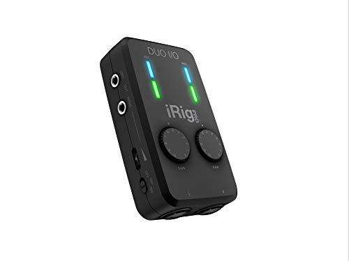 Audio interface
IK Multimedia iRig Pro Duo I/O USB audio interface, TRS balanced & headphones outputs, audio mixer to 24-bit, midi interface for music studio, recording, podcasting, streaming & social apps
Portable 2-channel USB-C audio interface used for mobile Biquadia field recording.
 $50.62Book
Loudspeaker Design Cookbook
Breakup modes, cone edge termination, and waveguide directivity index — chapters 7-9 explain the cone-breakup visualization and waveguide polar math this lab implements.
 $168.00Microphone
RØDE NT-USB+ Professional-Grade USB Condenser Microphone for Recording
USB condenser mic used for nymic testing.
 $8.99Audio
SABRENT USB External Stereo Sound Card Adapter, Plug & Play (AU-MMSA)
USB audio interface used in early Biquadia MEMS-mic prototyping.
 Microphone
Sennheiser Pro Audio Sennheiser Pro Audio Wireless Microphone System, Black (MKE600)
Wireless mic system used for akous's ambient/binaural field recording.
 $319.00Microphone
Shure MV7+ USB-C & XLR Podcast Dynamic Mic with Stand - Black
USB/XLR hybrid mic used building and testing nymic.
 $237.00Microphone
Shure MV88+ USB-C Video Kit Stereo Condenser Microphone
Portable stereo condenser mic kit used for Biquadia field/video capture.
 $98.00Headphones
Sony MDR7506 Professional Large Diaphragm Headphone
Reference studio headphones used for akous's binaural audio testing.
 $24.95Book
Testing Loudspeakers
Step-by-step measurement of Thiele-Small, K_ms(x), Le(x) — same nonlinearities the loudspeaker nonlinearity lab models with displacement-dependent Bl(x) and stiffness.
 $98.91Book
The Physics of Musical Instruments
Modal analysis of plates and strings with Bessel functions — root of Chladni plate eigenmodes and waveguide modal cutoff fc = c/2a this toolbox computes.
Prices shown were retrieved from the Amazon Product Advertising API on 8 October 2026 and are indicative only — the price and availability on Amazon at the time of purchase apply.
More gear across every app: the full Gear list →
Two gotchas worth knowing
The breakup_scale factor hides thickness, curvature, and edge condition
Real cone breakup depends on thickness (∝ t), curvature (curvilinear profiles raise fb by 20–40%), edge compliance (real surrounds lower fb by 15–25%), and anisotropy (woven materials differ 2× between warp and weft). The tool collapses all of this into a single material multiplier. Two 15 cm aluminum cones from different manufacturers can have fb anywhere from 5 kHz to 9 kHz. Use the override slider if you have a measured fb — the material selector is for qualitative exploration.
Frequency response plot is illustrative, not predictive
The synthetic SPL curve at the bottom uses procedural sine-modulation math, not actual acoustic radiation integrals. A real on-axis response includes: radiation impedance from the air load (which changes with frequency), the exact spatial integration of velocity over the cone surface weighted by Green's function, baffle diffraction, and the driver's electrical impedance interacting with the amplifier. The squiggles you see are qualitatively correct (peaks and dips grow past fb) but their exact dB values and frequencies are fabricated. For real response prediction, use a boundary element method (BEM) solver.
JavaScript — the mode shape solver
The core Bessel-mode displacement function mapping radius, angle, and a mode index to surface displacement. This is the heart of every colored triangle on the cone mesh. Sketch with elisions: the Bessel import is omitted and the running solver picks the mode from UI state rather than taking it as an argument.
Cone breakup modes — JavaScript
const MATERIALS = {
  paper:        { label: 'Paper',        E: 3,    rho: 700,  breakup_scale: 1.0 },
  polypropylene:{ label: 'Polypropylene', E: 1.5,  rho: 900,  breakup_scale: 0.7 },
  aluminum:     { label: 'Aluminum',      E: 70,   rho: 2700, breakup_scale: 2.5 },
  'carbon-fiber':{ label: 'Carbon fiber', E: 120,  rho: 1600, breakup_scale: 4.2 },
  kevlar:       { label: 'Kevlar',        E: 80,   rho: 1440, breakup_scale: 3.6 },
  titanium:     { label: 'Titanium',      E: 110,  rho: 4500, breakup_scale: 2.4 },
};

const breakupFreq = (material, diamCm) =>
  MATERIALS[material].breakup_scale * 2800 * (15 / diamCm);

const modeShape = (r, theta, mode) => {
  const rn = Math.min(1, Math.max(0, r));
  switch (mode) {
    case 1: return 1.0; // piston
    case 2: return besselJ(0, 3.8317 * rn); // J₀ first root
    case 3: return besselJ(0, 7.0156 * rn); // J₀ second root
    case 4: return (besselJ(1, 3.8317 * rn) / 0.5819) * Math.cos(theta);
    case 5: return (besselJ(2, 5.1356 * rn) / 0.486) * Math.cos(2 * theta);
    default: return 1.0;
  }
};

const computeDisplacement = (r, theta, f, fb, mode) => {
  const ratio = f / Math.max(1, fb);
  const pistonAmp = Math.max(0, 1 - ratio);
  const modalAmp = Math.pow(Math.max(0, ratio - 0.35), 1.2) * 1.5;
  return 0.35 * pistonAmp + modalAmp * modeShape(r, theta, mode);
};
Frequently asked questions
What does the breakup frequency depend on?
fb ∝ √(E/ρ) / D — stiffness (Young's modulus E) pushes it up, density (ρ) drags it down, and diameter (D) is the strongest lever (fb ∝ 1/D² for constant thickness, approximately 1/D here since effective t/R is treated as thin-shell). A 15 cm paper cone breaks up around 2.8 kHz; the same size in carbon fiber breaks up around 11.8 kHz. That's why tweeters are small and midranges use stiff materials.
Why does phase coherence drop even when the displacement pattern looks mild?
Phase coherence is |Σ e^(jφᵢ)| / N — a measure of how many points on the cone are moving in the same direction at the same time. Even a small modal contribution creates opposing rings. Once two regions 180° out of phase have comparable area, coherence drops fast. Below 40%, the on-axis cancellation is so severe that EQ cannot restore flat response — you need a physically stiffer cone.
Are Bessel functions really how real cones behave?
Only approximately. Real cones are curved (conical or curvilinear profiles), which stiffens the structure against radial modes. The edge condition in a real driver is compliant (surround + spider), not clamped. Dust caps add mass and stiffness. Anisotropic materials like woven carbon fiber have different stiffness along warp vs weft. The Bessel modes shown here give the correct qualitative pattern — central dome, then concentric nodal circles, then diametral splitting — but real frequencies differ by 20–50% from the ideal clamped-plate prediction.
Can I use this tool to pick a crossover frequency?
Yes, for quick intuition. Keep your crossover below 0.7·fb. If the breakup frequency is 2.8 kHz, cross no higher than ~2.0 kHz. If you must cross higher (e.g., a 2-way with a tweeter that can't go below 3 kHz), you need a driver with breakup above 4.3 kHz — select a stiffer material or smaller diameter in the tool and check. For production designs, always verify with polar measurements.
Why is paper often preferred despite its low breakup frequency?
Paper has high internal damping (loss factor η ≈ 0.04–0.08). When it breaks up, the modal peaks are gentle — only 2–4 dB. Aluminum has very low damping (η ≈ 0.001) — when it breaks up, resonance peaks can reach 10–15 dB and ring for many cycles. So paper's breakup is "softer" and more easily managed with simple EQ, while metal cones need notch filters precisely tuned to each breakup mode. The frequency response plot in this tool is illustrative and does not show damping — in reality, paper shows gentler peaks.
Shareable still
The instrument, captured—not illustrated.
This 16:9 frame is rendered from the real browser instrument above. It is the page's canonical preview for image search, link unfurls, and posts that need to show what the tool actually does.
Download 1280 × 720 JPEG